Analysis: Randomized block design

This is a function of the AgroR package for statistical analysis of experiments conducted in a randomized block and balanced design with a factor considering the fixed model. The function presents the option to use non-parametric method or transform the dataset.

DBC(
  trat,
  block,
  response,
  norm = "sw",
  homog = "bt",
  alpha.f = 0.05,
  alpha.t = 0.05,
  quali = TRUE,
  mcomp = "tukey",
  grau = 1,
  transf = 1,
  constant = 0,
  test = "parametric",
  geom = "bar",
  theme = theme_classic(),
  sup = NA,
  CV = TRUE,
  ylab = "response",
  xlab = "",
  textsize = 12,
  labelsize = 4,
  fill = "lightblue",
  angle = 0,
  family = "sans",
  dec = 3,
  width.column = NULL,
  width.bar = 0.3,
  addmean = TRUE,
  errorbar = TRUE,
  posi = "top",
  point = "mean_sd",
  angle.label = 0,
  ylim = NA
)

Arguments

trat

Numerical or complex vector with treatments

block

Numerical or complex vector with blocks

response

Numerical vector containing the response of the experiment.

norm

Error normality test (default is Shapiro-Wilk)

homog

Homogeneity test of variances (default is Bartlett)

alpha.f

Level of significance of the F test (default is 0.05)

alpha.t

Significance level of the multiple comparison test (default is 0.05)

quali

Defines whether the factor is quantitative or qualitative (default is qualitative)

mcomp

Multiple comparison test (Tukey (default), LSD, Scott-Knott and Duncan)

grau

Degree of polynomial in case of quantitative factor (default is 1)

transf

Applies data transformation (default is 1; for log consider 0; `angular` for angular transformation)

constant

Add a constant for transformation (enter value)

test

"parametric" - Parametric test or "noparametric" - non-parametric test

geom

graph type (columns, boxes or segments)

theme

ggplot2 theme (default is theme_classic())

sup

Number of units above the standard deviation or average bar on the graph

CV

Plotting the coefficient of variation and p-value of Anova (default is TRUE)

ylab

Variable response name (Accepts the expression() function)

xlab

Treatments name (Accepts the expression() function)

textsize

Font size

labelsize

Label size

fill

Defines chart color (to generate different colors for different treatments, define fill = "trat")

angle

x-axis scale text rotation

family

Font family

dec

Number of cells

width.column

Width column if geom="bar"

width.bar

Width errorbar

addmean

Plot the average value on the graph (default is TRUE)

errorbar

Plot the standard deviation bar on the graph (In the case of a segment and column graph) - default is TRUE

posi

Legend position

point

Defines whether to plot mean ("mean"), mean with standard deviation ("mean_sd" - default) or mean with standard error ("mean_se"). For parametric test it is possible to plot the square root of QMres (mean_qmres).

angle.label

label angle

ylim

Define a numerical sequence referring to the y scale. You can use a vector or the `seq` command.

Value

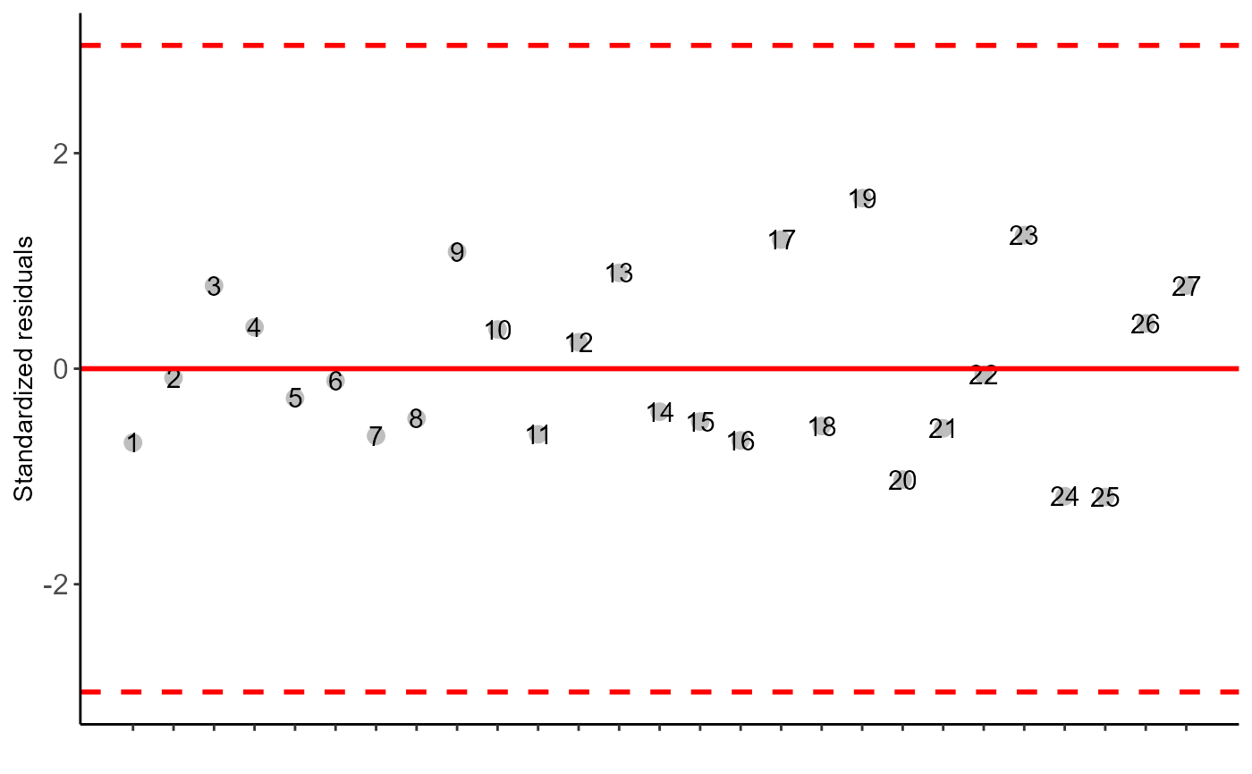
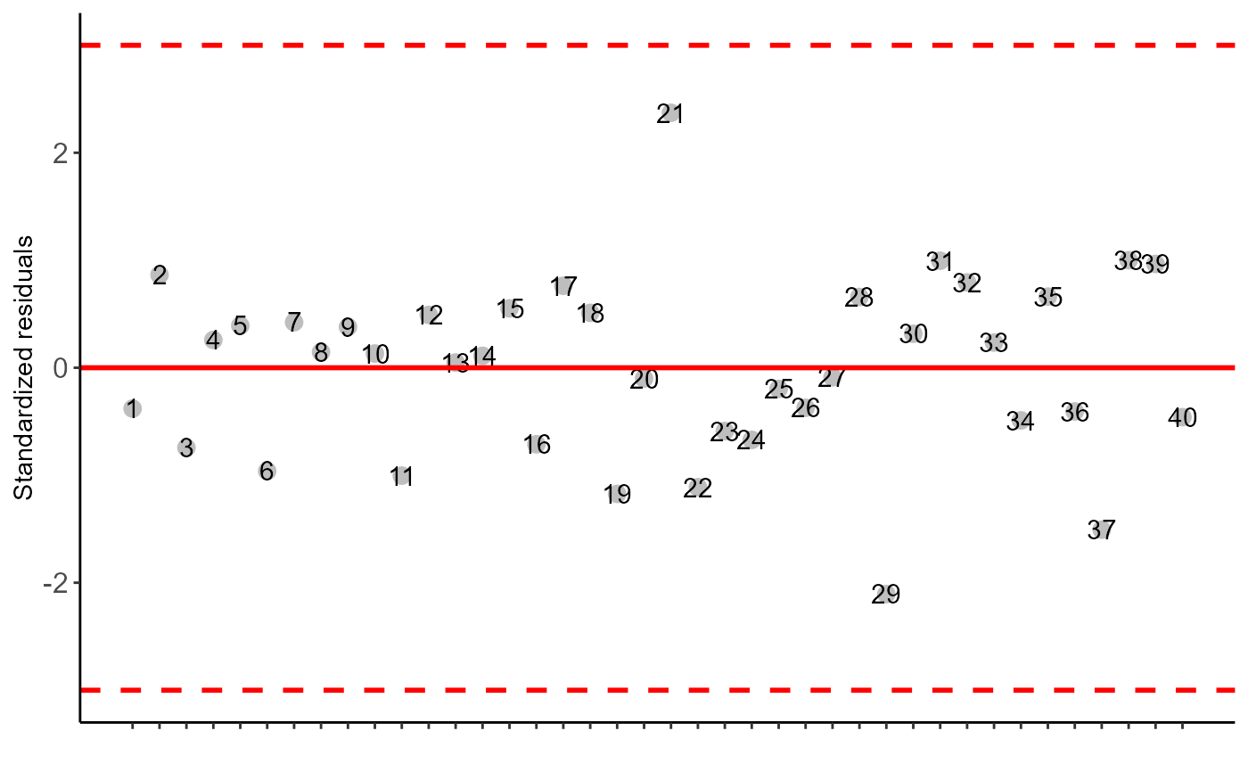
The table of analysis of variance, the test of normality of errors (Shapiro-Wilk ("sw"), Lilliefors ("li"), Anderson-Darling ("ad"), Cramer-von Mises ("cvm"), Pearson ("pearson") and Shapiro-Francia ("sf")), the test of homogeneity of variances (Bartlett ("bt") or Levene ("levene")), the test of independence of Durbin-Watson errors, the test of multiple comparisons (Tukey ("tukey"), LSD ("lsd"), Scott-Knott ("sk") or Duncan ("duncan")) or adjustment of regression models up to grade 3 polynomial, in the case of quantitative treatments. Non-parametric analysis can be used by the Friedman test. The column, segment or box chart for qualitative treatments is also returned. The function also returns a standardized residual plot.

Note

Enable ggplot2 package to change theme argument.

The ordering of the graph is according to the sequence in which the factor levels are arranged in the data sheet. The bars of the column and segment graphs are standard deviation.

CV and p-value of the graph indicate coefficient of variation and p-value of the F test of the analysis of variance.

In the final output when transformation (transf argument) is different from 1, the columns resp and respo in the mean test are returned, indicating transformed and non-transformed mean, respectively.

References

Principles and procedures of statistics a biometrical approach Steel, Torry and Dickey. Third Edition 1997

Multiple comparisons theory and methods. Departament of statistics the Ohio State University. USA, 1996. Jason C. Hsu. Chapman Hall/CRC.

Practical Nonparametrics Statistics. W.J. Conover, 1999

Ramalho M.A.P., Ferreira D.F., Oliveira A.C. 2000. Experimentacao em Genetica e Melhoramento de Plantas. Editora UFLA.

Scott R.J., Knott M. 1974. A cluster analysis method for grouping mans in the analysis of variance. Biometrics, 30, 507-512.

Mendiburu, F., and de Mendiburu, M. F. (2019). Package ‘agricolae’. R Package, Version, 1-2.

See also

DIC, DQL

Author

Gabriel Danilo Shimizu, shimizu@uel.br

Leandro Simoes Azeredo Goncalves

Rodrigo Yudi Palhaci Marubayashi

Examples

library(AgroR)

#=============================
# Example laranja
#=============================
data(laranja)
attach(laranja)
#> The following objects are masked from aristolochia:
#> 
#>     resp, trat
#> The following objects are masked from cloro:
#> 
#>     bloco, resp
#> The following objects are masked from passiflora:
#> 
#>     bloco, trat
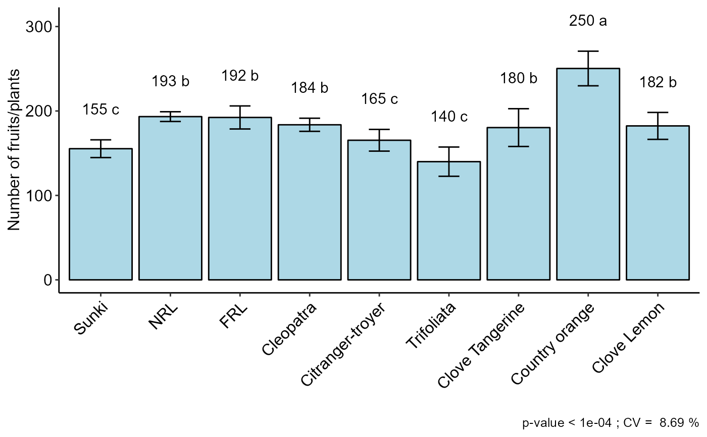
DBC(trat, bloco, resp, mcomp = "sk", angle=45, ylab = "Number of fruits/plants")
#> 
#> -----------------------------------------------------------------
#> Normality of errors
#> -----------------------------------------------------------------
#>                          Method Statistic  p.value
#>  Shapiro-Wilk normality test(W) 0.9475889 0.187264
#> 
#> As the calculated p-value is greater than the 5% significance level, hypothesis H0 is not rejected. Therefore, errors can be considered normal
#> 
#> -----------------------------------------------------------------
#> Homogeneity of Variances
#> -----------------------------------------------------------------
#>                               Method Statistic p.value
#>  Bartlett test(Bartlett's K-squared)  4.036888 0.85378
#> 
#> As the calculated p-value is greater than the 5% significance level, hypothesis H0 is not rejected. Therefore, the variances can be considered homogeneous
#> 
#> -----------------------------------------------------------------
#> Independence from errors
#> -----------------------------------------------------------------
#>                  Method Statistic   p.value
#>  Durbin-Watson test(DW)  2.324604 0.2484349
#> 
#> As the calculated p-value is greater than the 5% significance level, hypothesis H0 is not rejected. Therefore, errors can be considered independent
#> 
#> -----------------------------------------------------------------
#> Additional Information
#> -----------------------------------------------------------------
#> 
#> CV (%) =  8.69
#> MStrat/MST =  0.91
#> Mean =  182.5556
#> Median =  183
#> Possible outliers =  No discrepant point
#> 
#> -----------------------------------------------------------------
#> Analysis of Variance
#> -----------------------------------------------------------------
#>           Df      Sum Sq    Mean.Sq     F value        Pr(F)
#> trat       8 22981.33333 2872.66667 11.41142069 2.636524e-05
#> bloco      2    33.55556   16.77778  0.06664828 9.357825e-01
#> Residuals 16  4027.77778  251.73611                         
#> 
#> As the calculated p-value, it is less than the 5% significance level. The hypothesis H0 of equality of means is rejected. Therefore, at least two treatments differ

#> 
#> -----------------------------------------------------------------
#> Multiple Comparison Test: Scott-Knott
#> -----------------------------------------------------------------
#>                      resp groups
#> Country orange   250.3333      a
#> NRL              193.3333      b
#> FRL              192.3333      b
#> Cleopatra        183.6667      b
#> Clove Lemon      182.3333      b
#> Clove Tangerine  180.3333      b
#> Citranger-troyer 165.3333      c
#> Sunki            155.3333      c
#> Trifoliata       140.0000      c
#> 


#=============================
# Friedman test
#=============================
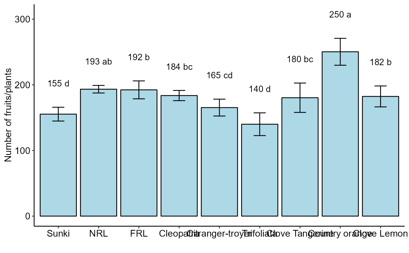
DBC(trat, bloco, resp, test="noparametric", ylab = "Number of fruits/plants")
#> 
#> 
#> -----------------------------------------------------------------
#> Statistics
#> -----------------------------------------------------------------
#>      Chisq Df    p.chisq        F DFerror          p.F  t.value      LSD
#>   19.30726  8 0.01330002 8.228571      16 0.0001991497 2.119905 7.680087
#> 
#> 
#> -----------------------------------------------------------------
#> Parameters
#> -----------------------------------------------------------------
#>       test name.t ntr alpha
#>   Friedman   trat   9  0.05
#> 
#> 
#> -----------------------------------------------------------------
#> Multiple Comparison Test: LSD
#> -----------------------------------------------------------------
#>                      Mean        SD Rank Groups
#> Citranger-troyer 165.3333 12.858201  8.5     cd
#> Cleopatra        183.6667  7.767453 16.0     bc
#> Clove Lemon      182.3333 15.947832 17.5      b
#> Clove Tangerine  180.3333 22.368132 16.0     bc
#> Country orange   250.3333 20.502032 27.0      a
#> FRL              192.3333 13.650397 19.0      b
#> NRL              193.3333  5.773503 20.5     ab
#> Sunki            155.3333 10.503968  6.0      d
#> Trifoliata       140.0000 17.320508  4.5      d


#=============================
# Example soybean
#=============================
data(soybean)
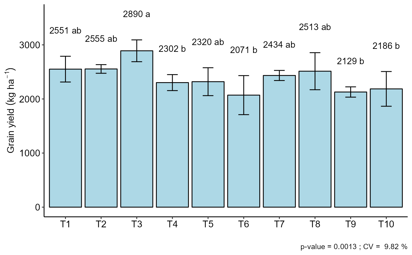
with(soybean, DBC(cult, bloc, prod,
                  ylab=expression("Grain yield"~(kg~ha^-1))))
#> 
#> -----------------------------------------------------------------
#> Normality of errors
#> -----------------------------------------------------------------
#>                          Method Statistic   p.value
#>  Shapiro-Wilk normality test(W)   0.97649 0.5613183
#> 
#> As the calculated p-value is greater than the 5% significance level, hypothesis H0 is not rejected. Therefore, errors can be considered normal
#> 
#> -----------------------------------------------------------------
#> Homogeneity of Variances
#> -----------------------------------------------------------------
#>                               Method Statistic   p.value
#>  Bartlett test(Bartlett's K-squared)   9.54102 0.3889021
#> 
#> As the calculated p-value is greater than the 5% significance level, hypothesis H0 is not rejected. Therefore, the variances can be considered homogeneous
#> 
#> -----------------------------------------------------------------
#> Independence from errors
#> -----------------------------------------------------------------
#>                  Method Statistic   p.value
#>  Durbin-Watson test(DW)  2.484876 0.5578071
#> 
#> As the calculated p-value is greater than the 5% significance level, hypothesis H0 is not rejected. Therefore, errors can be considered independent
#> 
#> -----------------------------------------------------------------
#> Additional Information
#> -----------------------------------------------------------------
#> 
#> CV (%) =  9.82
#> MStrat/MST =  0.67
#> Mean =  2395.2
#> Median =  2444
#> Possible outliers =  No discrepant point
#> 
#> -----------------------------------------------------------------
#> Analysis of Variance
#> -----------------------------------------------------------------
#>           Df    Sum Sq   Mean.Sq  F value       Pr(F)
#> trat       9 2178702.9 242078.10 4.374765 0.001344107
#> bloco      3  187633.4  62544.47 1.130285 0.354392706
#> Residuals 27 1494048.1  55335.11                     
#> 
#> As the calculated p-value, it is less than the 5% significance level. The hypothesis H0 of equality of means is rejected. Therefore, at least two treatments differ

#> 
#> -----------------------------------------------------------------
#> Multiple Comparison Test: Tukey HSD
#> -----------------------------------------------------------------
#>        resp groups
#> T3  2890.50      a
#> T2  2554.75     ab
#> T1  2551.25     ab
#> T8  2513.25     ab
#> T7  2434.25     ab
#> T5  2319.50     ab
#> T4  2302.50      b
#> T10 2186.25      b
#> T9  2128.75      b
#> T6  2071.00      b
#>