Graph: Point graph for one factor model 2
seg_graph2.RdThis is a function of the point graph for one factor
seg_graph2(
  model,
  theme = theme_gray(),
  pointsize = 4,
  pointshape = 16,
  horiz = TRUE,
  vjust = -0.6
)
Arguments
- model
DIC, DBC or DQL object
- theme
ggplot2 theme
- pointsize
Point size
- pointshape
Format point (default is 16)
- horiz
Horizontal Column (default is TRUE)
- vjust
vertical adjusted
Value
Returns a point chart for one factor
See also
Examples
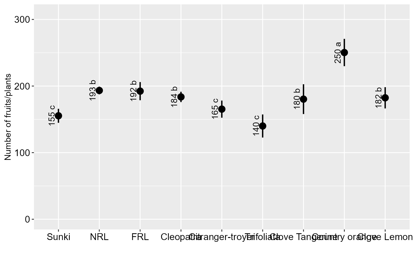
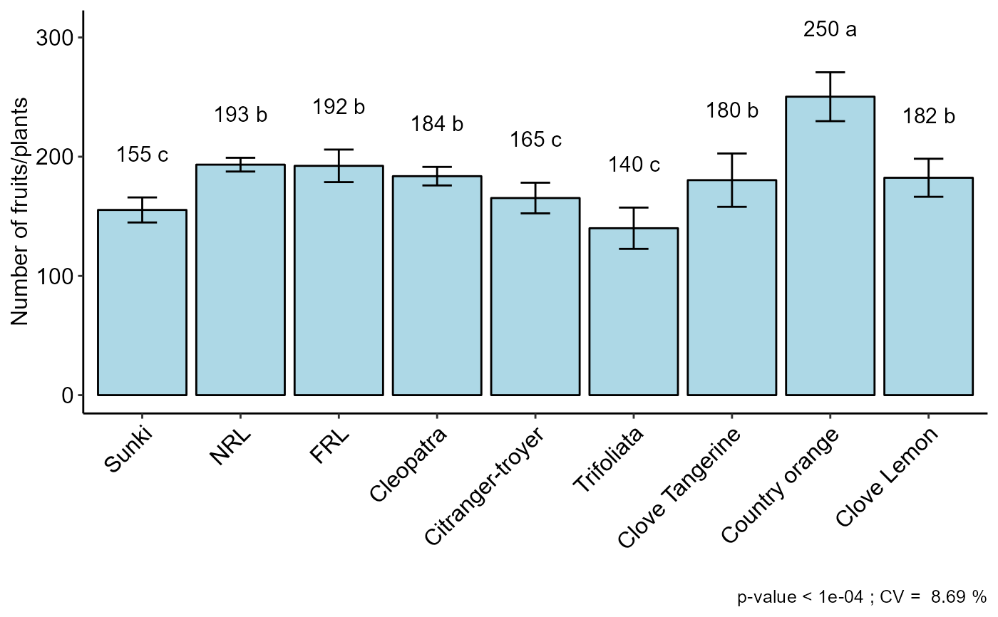
data("laranja")
a=with(laranja, DBC(trat, bloco, resp,
mcomp = "sk",angle=45,
ylab = "Number of fruits/plants"))
#>
#> -----------------------------------------------------------------
#> Normality of errors
#> -----------------------------------------------------------------
#> Method Statistic p.value
#> Shapiro-Wilk normality test(W) 0.9475889 0.187264
#>
#> As the calculated p-value is greater than the 5% significance level, hypothesis H0 is not rejected. Therefore, errors can be considered normal
#>
#> -----------------------------------------------------------------
#> Homogeneity of Variances
#> -----------------------------------------------------------------
#> Method Statistic p.value
#> Bartlett test(Bartlett's K-squared) 4.036888 0.85378
#>
#> As the calculated p-value is greater than the 5% significance level, hypothesis H0 is not rejected. Therefore, the variances can be considered homogeneous
#>
#> -----------------------------------------------------------------
#> Independence from errors
#> -----------------------------------------------------------------
#> Method Statistic p.value
#> Durbin-Watson test(DW) 2.324604 0.2484349
#>
#> As the calculated p-value is greater than the 5% significance level, hypothesis H0 is not rejected. Therefore, errors can be considered independent
#>
#> -----------------------------------------------------------------
#> Additional Information
#> -----------------------------------------------------------------
#>
#> CV (%) = 8.69
#> MStrat/MST = 0.91
#> Mean = 182.5556
#> Median = 183
#> Possible outliers = No discrepant point
#>
#> -----------------------------------------------------------------
#> Analysis of Variance
#> -----------------------------------------------------------------
#> Df Sum Sq Mean.Sq F value Pr(F)
#> trat 8 22981.33333 2872.66667 11.41142069 2.636524e-05
#> bloco 2 33.55556 16.77778 0.06664828 9.357825e-01
#> Residuals 16 4027.77778 251.73611
#>
#> As the calculated p-value, it is less than the 5% significance level. The hypothesis H0 of equality of means is rejected. Therefore, at least two treatments differ
 #>
#> -----------------------------------------------------------------
#> Multiple Comparison Test: Scott-Knott
#> -----------------------------------------------------------------
#> resp groups
#> Country orange 250.3333 a
#> NRL 193.3333 b
#> FRL 192.3333 b
#> Cleopatra 183.6667 b
#> Clove Lemon 182.3333 b
#> Clove Tangerine 180.3333 b
#> Citranger-troyer 165.3333 c
#> Sunki 155.3333 c
#> Trifoliata 140.0000 c
#>
#>
#> -----------------------------------------------------------------
#> Multiple Comparison Test: Scott-Knott
#> -----------------------------------------------------------------
#> resp groups
#> Country orange 250.3333 a
#> NRL 193.3333 b
#> FRL 192.3333 b
#> Cleopatra 183.6667 b
#> Clove Lemon 182.3333 b
#> Clove Tangerine 180.3333 b
#> Citranger-troyer 165.3333 c
#> Sunki 155.3333 c
#> Trifoliata 140.0000 c
#>
 seg_graph2(a,horiz = FALSE)