Utils: Summary of Analysis of Variance and Test of Means
summarise_anova.RdSummarizes the output of the analysis of variance and the multiple comparisons test for completely randomized (DIC), randomized block (DBC) and Latin square (DQL) designs.
summarise_anova(analysis, inf = "p", design = "DIC", round = 3, divisor = TRUE)Arguments
- analysis
List with the analysis outputs of the DIC, DBC, DQL, FAT2DIC, FAT2DBC, PSUBDIC and PSUBDBC functions
- inf
Analysis of variance information (can be "p", "f", "QM" or "SQ")
- design
Type of experimental project (DIC, DBC, DQL, FAT2DIC, FAT2DBC, PSUBDIC or PSUBDBC)
- round
Number of decimal places
- divisor
Add divider between columns
Note
Adding table divider can help to build tables in microsoft word. Copy console output, paste into MS Word, Insert, Table, Convert text to table, Separated text into:, Other: |.
The column names in the final output are imported from the ylab argument within each function.
This function is only for declared qualitative factors. In the case of a quantitative factor and the other qualitative in projects with two factors, this function will not work.
Triple factorials and split-split-plot do not work in this function.
Examples
library(AgroR)
#=====================================
# DIC
#=====================================
data(pomegranate)
attach(pomegranate)
#> The following object is masked from mirtilo:
#>
#> trat
#> The following object is masked from simulate3:
#>
#> trat
#> The following object is masked from simulate1:
#>
#> trat
#> The following object is masked from aristolochia (pos = 12):
#>
#> trat
#> The following object is masked from simulate2:
#>
#> trat
#> The following object is masked from laranja:
#>
#> trat
#> The following object is masked from aristolochia (pos = 15):
#>
#> trat
#> The following object is masked from passiflora:
#>
#> trat
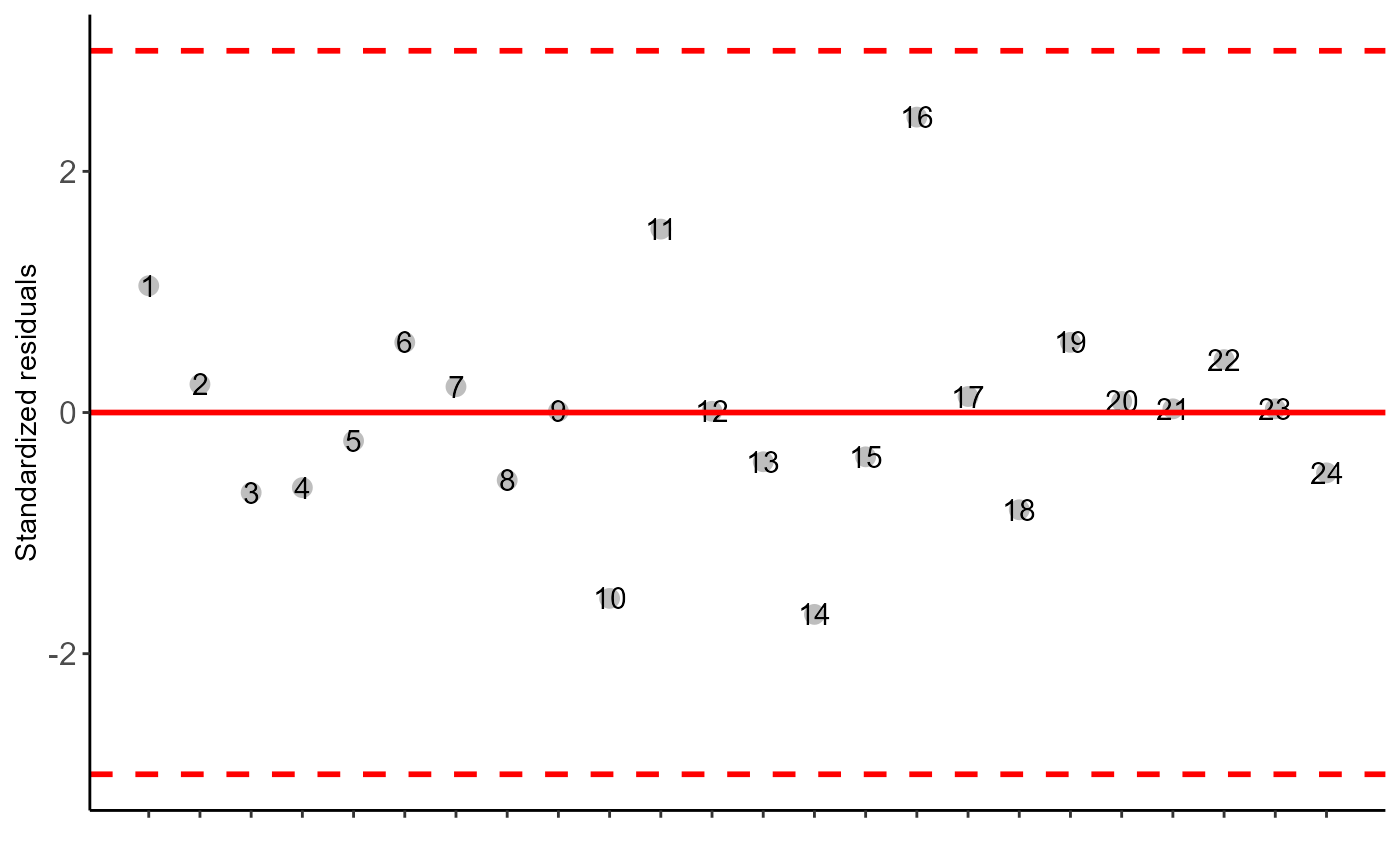
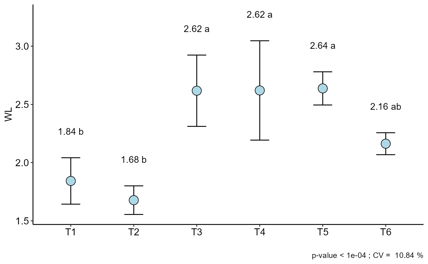
a=DIC(trat, WL, geom = "point", ylab = "WL")
#>
#> -----------------------------------------------------------------
#> Normality of errors
#> -----------------------------------------------------------------
#> Method Statistic p.value
#> Shapiro-Wilk normality test(W) 0.9448293 0.2087967
#>
#> As the calculated p-value is greater than the 5% significance level, hypothesis H0 is not rejected. Therefore, errors can be considered normal
#>
#> -----------------------------------------------------------------
#> Homogeneity of Variances
#> -----------------------------------------------------------------
#> Method Statistic p.value
#> Bartlett test(Bartlett's K-squared) 8.568274 0.1275737
#>
#> As the calculated p-value is greater than the 5% significance level,hypothesis H0 is not rejected. Therefore, the variances can be considered homogeneous
#>
#> -----------------------------------------------------------------
#> Independence from errors
#> -----------------------------------------------------------------
#> Method Statistic p.value
#> Durbin-Watson test(DW) 2.104821 0.1924474
#>
#> As the calculated p-value is greater than the 5% significance level, hypothesis H0 is not rejected. Therefore, errors can be considered independent
#>
#> -----------------------------------------------------------------
#> Additional Information
#> -----------------------------------------------------------------
#>
#> CV (%) = 10.84
#> MStrat/MST = 0.92
#> Mean = 2.2596
#> Median = 2.225
#> Possible outliers = No discrepant point
#>
#> -----------------------------------------------------------------
#> Analysis of Variance
#> -----------------------------------------------------------------
#> Df Sum Sq Mean.Sq F value Pr(F)
#> trat 5 3.692121 0.73842417 12.31191 2.723541e-05
#> Residuals 18 1.079575 0.05997639
#>
#>
#> As the calculated p-value, it is less than the 5% significance level.The hypothesis H0 of equality of means is rejected. Therefore, at least two treatments differ
#>
#>
#> -----------------------------------------------------------------
#> Multiple Comparison Test: Tukey HSD
#> -----------------------------------------------------------------
#> resp groups
#> T5 2.6375 a
#> T4 2.6200 a
#> T3 2.6175 a
#> T6 2.1625 ab
#> T1 1.8425 b
#> T2 1.6775 b
#>
#>
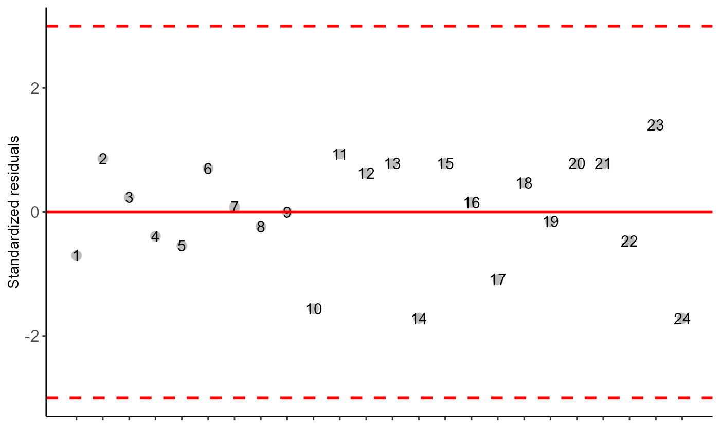
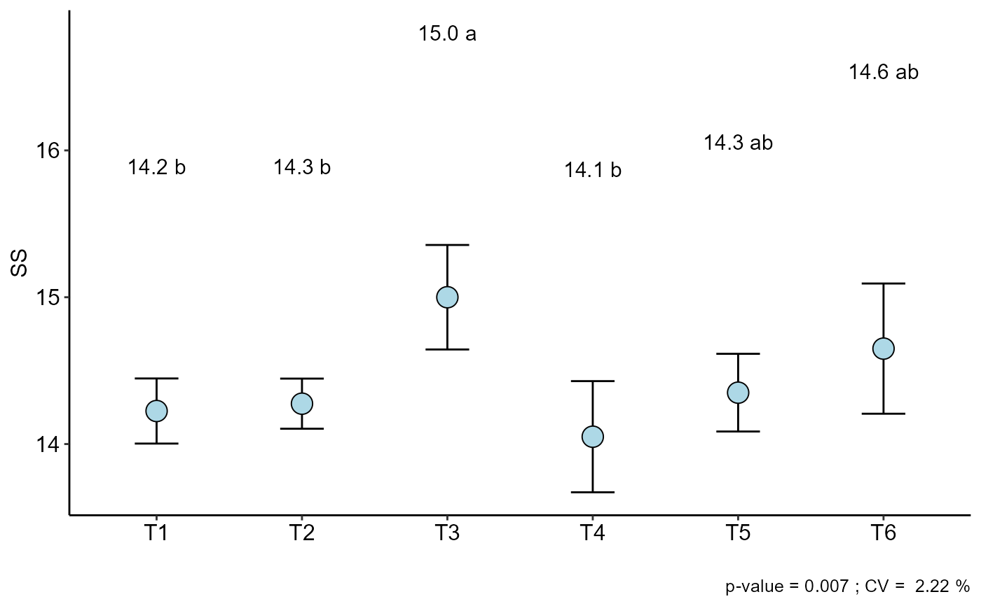
 b=DIC(trat, SS, geom = "point", ylab="SS")
#>
#> -----------------------------------------------------------------
#> Normality of errors
#> -----------------------------------------------------------------
#> Method Statistic p.value
#> Shapiro-Wilk normality test(W) 0.9286937 0.09115023
#>
#> As the calculated p-value is greater than the 5% significance level, hypothesis H0 is not rejected. Therefore, errors can be considered normal
#>
#> -----------------------------------------------------------------
#> Homogeneity of Variances
#> -----------------------------------------------------------------
#> Method Statistic p.value
#> Bartlett test(Bartlett's K-squared) 3.118359 0.6817441
#>
#> As the calculated p-value is greater than the 5% significance level,hypothesis H0 is not rejected. Therefore, the variances can be considered homogeneous
#>
#> -----------------------------------------------------------------
#> Independence from errors
#> -----------------------------------------------------------------
#> Method Statistic p.value
#> Durbin-Watson test(DW) 2.618225 0.7051835
#>
#> As the calculated p-value is greater than the 5% significance level, hypothesis H0 is not rejected. Therefore, errors can be considered independent
#>
#> -----------------------------------------------------------------
#> Additional Information
#> -----------------------------------------------------------------
#>
#> CV (%) = 2.22
#> MStrat/MST = 0.82
#> Mean = 14.425
#> Median = 14.3
#> Possible outliers = No discrepant point
#>
#> -----------------------------------------------------------------
#> Analysis of Variance
#> -----------------------------------------------------------------
#> Df Sum Sq Mean.Sq F value Pr(F)
#> trat 5 2.360 0.4720 4.604878 0.007008811
#> Residuals 18 1.845 0.1025
#>
#>
#> As the calculated p-value, it is less than the 5% significance level.The hypothesis H0 of equality of means is rejected. Therefore, at least two treatments differ
#>
#>
#> -----------------------------------------------------------------
#> Multiple Comparison Test: Tukey HSD
#> -----------------------------------------------------------------
#> resp groups
#> T3 15.000 a
#> T6 14.650 ab
#> T5 14.350 ab
#> T2 14.275 b
#> T1 14.225 b
#> T4 14.050 b
#>
#>
b=DIC(trat, SS, geom = "point", ylab="SS")
#>
#> -----------------------------------------------------------------
#> Normality of errors
#> -----------------------------------------------------------------
#> Method Statistic p.value
#> Shapiro-Wilk normality test(W) 0.9286937 0.09115023
#>
#> As the calculated p-value is greater than the 5% significance level, hypothesis H0 is not rejected. Therefore, errors can be considered normal
#>
#> -----------------------------------------------------------------
#> Homogeneity of Variances
#> -----------------------------------------------------------------
#> Method Statistic p.value
#> Bartlett test(Bartlett's K-squared) 3.118359 0.6817441
#>
#> As the calculated p-value is greater than the 5% significance level,hypothesis H0 is not rejected. Therefore, the variances can be considered homogeneous
#>
#> -----------------------------------------------------------------
#> Independence from errors
#> -----------------------------------------------------------------
#> Method Statistic p.value
#> Durbin-Watson test(DW) 2.618225 0.7051835
#>
#> As the calculated p-value is greater than the 5% significance level, hypothesis H0 is not rejected. Therefore, errors can be considered independent
#>
#> -----------------------------------------------------------------
#> Additional Information
#> -----------------------------------------------------------------
#>
#> CV (%) = 2.22
#> MStrat/MST = 0.82
#> Mean = 14.425
#> Median = 14.3
#> Possible outliers = No discrepant point
#>
#> -----------------------------------------------------------------
#> Analysis of Variance
#> -----------------------------------------------------------------
#> Df Sum Sq Mean.Sq F value Pr(F)
#> trat 5 2.360 0.4720 4.604878 0.007008811
#> Residuals 18 1.845 0.1025
#>
#>
#> As the calculated p-value, it is less than the 5% significance level.The hypothesis H0 of equality of means is rejected. Therefore, at least two treatments differ
#>
#>
#> -----------------------------------------------------------------
#> Multiple Comparison Test: Tukey HSD
#> -----------------------------------------------------------------
#> resp groups
#> T3 15.000 a
#> T6 14.650 ab
#> T5 14.350 ab
#> T2 14.275 b
#> T1 14.225 b
#> T4 14.050 b
#>
#>
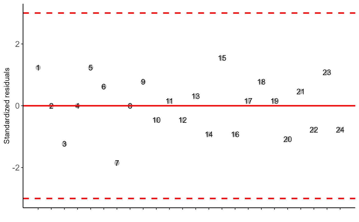
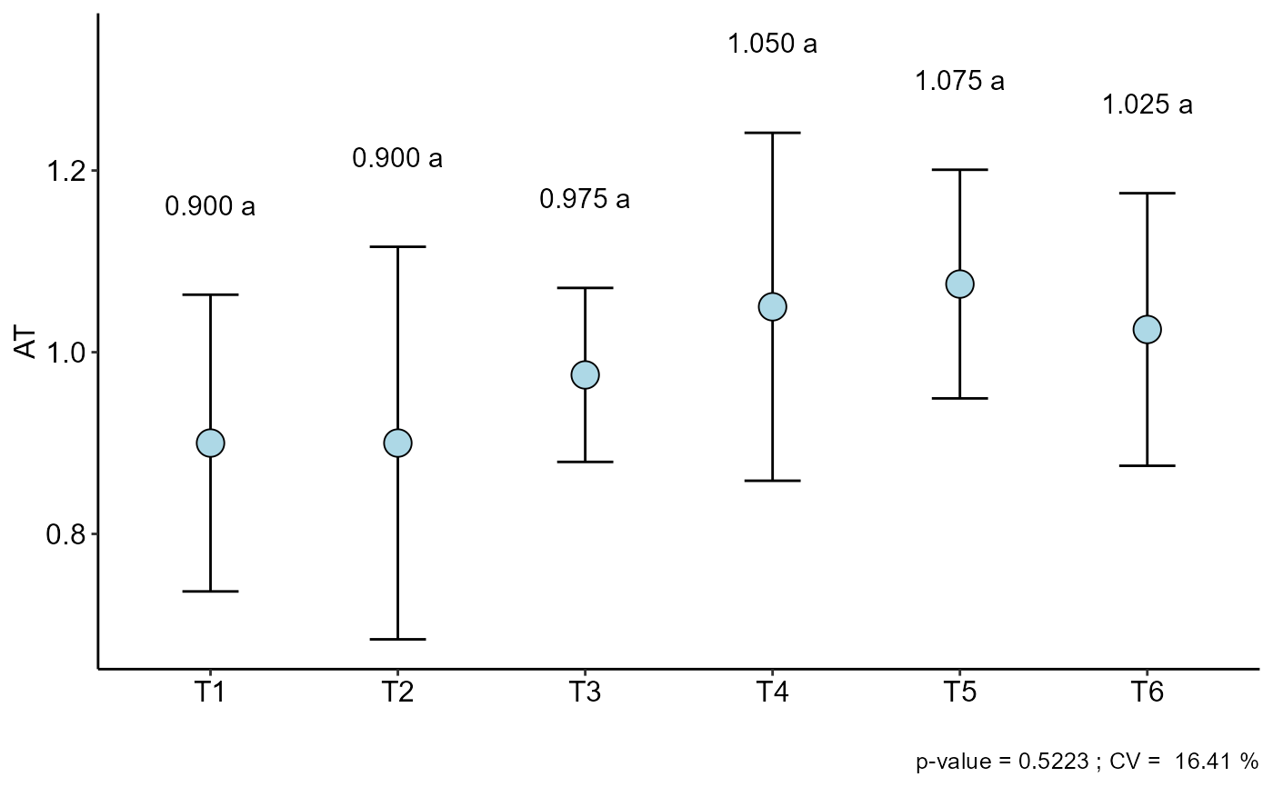
 c=DIC(trat, AT, geom = "point", ylab = "AT")
#>
#> -----------------------------------------------------------------
#> Normality of errors
#> -----------------------------------------------------------------
#> Method Statistic p.value
#> Shapiro-Wilk normality test(W) 0.9757571 0.8067715
#>
#> As the calculated p-value is greater than the 5% significance level, hypothesis H0 is not rejected. Therefore, errors can be considered normal
#>
#> -----------------------------------------------------------------
#> Homogeneity of Variances
#> -----------------------------------------------------------------
#> Method Statistic p.value
#> Bartlett test(Bartlett's K-squared) 2.088676 0.8367439
#>
#> As the calculated p-value is greater than the 5% significance level,hypothesis H0 is not rejected. Therefore, the variances can be considered homogeneous
#>
#> -----------------------------------------------------------------
#> Independence from errors
#> -----------------------------------------------------------------
#> Method Statistic p.value
#> Durbin-Watson test(DW) 2.633598 0.7201694
#>
#> As the calculated p-value is greater than the 5% significance level, hypothesis H0 is not rejected. Therefore, errors can be considered independent
#>
#> -----------------------------------------------------------------
#> Additional Information
#> -----------------------------------------------------------------
#>
#> CV (%) = 16.41
#> MStrat/MST = 0.46
#> Mean = 0.9875
#> Median = 0.95
#> Possible outliers = No discrepant point
#>
#> -----------------------------------------------------------------
#> Analysis of Variance
#> -----------------------------------------------------------------
#> Df Sum Sq Mean.Sq F value Pr(F)
#> trat 5 0.11375 0.02275 0.8666667 0.5222835
#> Residuals 18 0.47250 0.02625
#>
#>
#> As the calculated p-value is greater than the 5% significance level, H0 is not rejected
#>
#>
#> -----------------------------------------------------------------
#> Multiple Comparison Test: Tukey HSD
#> -----------------------------------------------------------------
#> [1] "H0 is not rejected"
#>
#>
c=DIC(trat, AT, geom = "point", ylab = "AT")
#>
#> -----------------------------------------------------------------
#> Normality of errors
#> -----------------------------------------------------------------
#> Method Statistic p.value
#> Shapiro-Wilk normality test(W) 0.9757571 0.8067715
#>
#> As the calculated p-value is greater than the 5% significance level, hypothesis H0 is not rejected. Therefore, errors can be considered normal
#>
#> -----------------------------------------------------------------
#> Homogeneity of Variances
#> -----------------------------------------------------------------
#> Method Statistic p.value
#> Bartlett test(Bartlett's K-squared) 2.088676 0.8367439
#>
#> As the calculated p-value is greater than the 5% significance level,hypothesis H0 is not rejected. Therefore, the variances can be considered homogeneous
#>
#> -----------------------------------------------------------------
#> Independence from errors
#> -----------------------------------------------------------------
#> Method Statistic p.value
#> Durbin-Watson test(DW) 2.633598 0.7201694
#>
#> As the calculated p-value is greater than the 5% significance level, hypothesis H0 is not rejected. Therefore, errors can be considered independent
#>
#> -----------------------------------------------------------------
#> Additional Information
#> -----------------------------------------------------------------
#>
#> CV (%) = 16.41
#> MStrat/MST = 0.46
#> Mean = 0.9875
#> Median = 0.95
#> Possible outliers = No discrepant point
#>
#> -----------------------------------------------------------------
#> Analysis of Variance
#> -----------------------------------------------------------------
#> Df Sum Sq Mean.Sq F value Pr(F)
#> trat 5 0.11375 0.02275 0.8666667 0.5222835
#> Residuals 18 0.47250 0.02625
#>
#>
#> As the calculated p-value is greater than the 5% significance level, H0 is not rejected
#>
#>
#> -----------------------------------------------------------------
#> Multiple Comparison Test: Tukey HSD
#> -----------------------------------------------------------------
#> [1] "H0 is not rejected"
#>
#>
 summarise_anova(analysis = list(a,b,c), divisor = TRUE)
#> | WL | SS | AT |
#> T1 | 1.842 b | 14.225 b | 0.9 a |
#> T2 | 1.678 b | 14.275 b | 0.9 a |
#> T3 | 2.618 a | 15 a | 0.975 a |
#> T4 | 2.62 a | 14.05 b | 1.05 a |
#> T5 | 2.638 a | 14.35 ab | 1.075 a |
#> T6 | 2.163 ab | 14.65 ab | 1.025 a |
#> CV(%) | 10.838 | 2.219 | 16.407 |
#> p-value | p<0.001 | 0.007 | 0.522 |
#> Transformation | No transf | No transf | No transf |
library(knitr)
kable(summarise_anova(analysis = list(a,b,c), divisor = FALSE))
#>
#>
#> | |WL |SS |AT |
#> |:--------------|:---------|:---------|:---------|
#> |T1 |1.842 b |14.225 b |0.9 a |
#> |T2 |1.678 b |14.275 b |0.9 a |
#> |T3 |2.618 a |15 a |0.975 a |
#> |T4 |2.62 a |14.05 b |1.05 a |
#> |T5 |2.638 a |14.35 ab |1.075 a |
#> |T6 |2.163 ab |14.65 ab |1.025 a |
#> |CV(%) |10.838 |2.219 |16.407 |
#> |p-value |p<0.001 |0.007 |0.522 |
#> |Transformation |No transf |No transf |No transf |
#=====================================
# DBC
#=====================================
data(soybean)
attach(soybean)
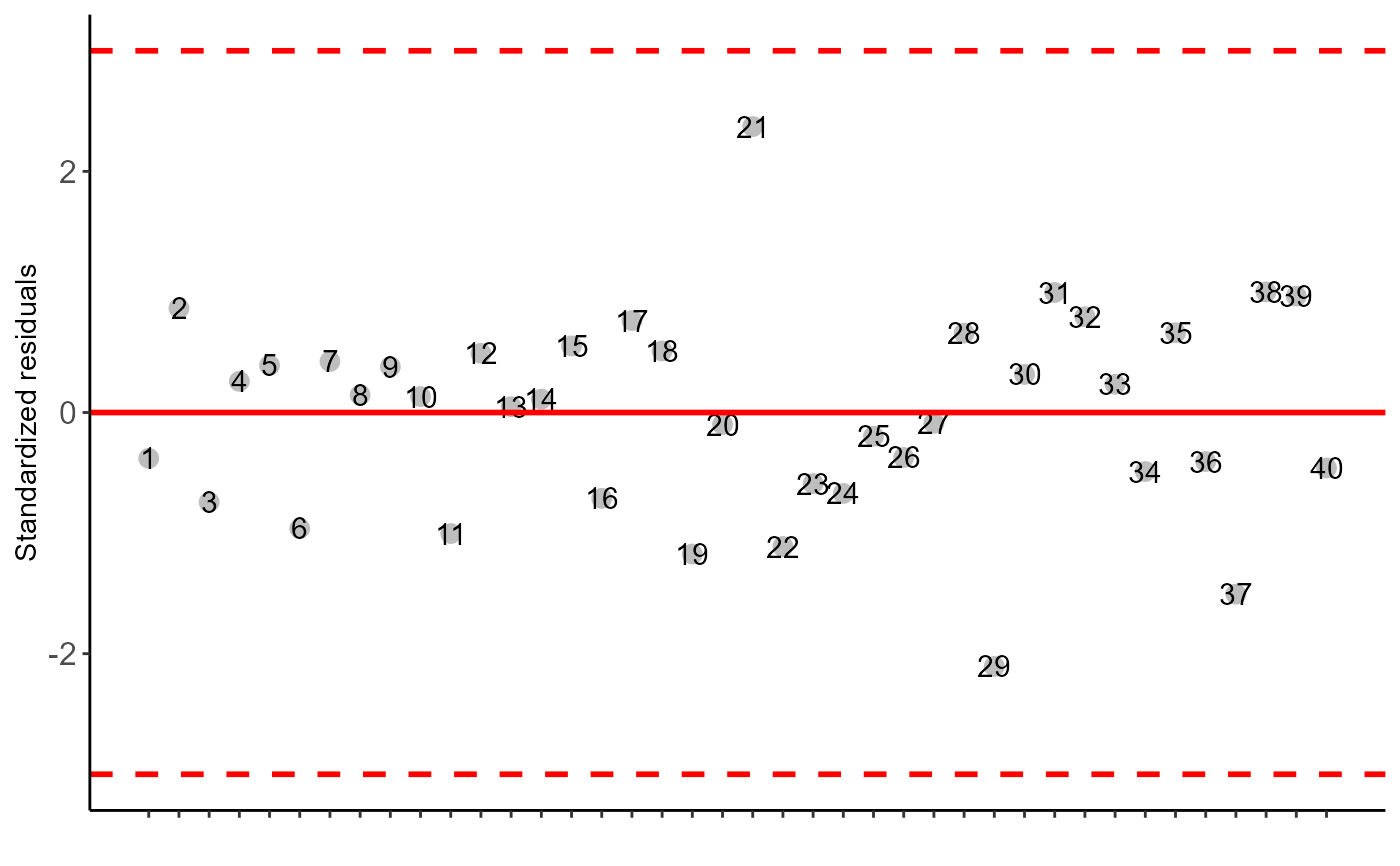
a=DBC(cult,bloc,prod,ylab = "Yield")
#>
#> -----------------------------------------------------------------
#> Normality of errors
#> -----------------------------------------------------------------
#> Method Statistic p.value
#> Shapiro-Wilk normality test(W) 0.97649 0.5613183
#>
#> As the calculated p-value is greater than the 5% significance level, hypothesis H0 is not rejected. Therefore, errors can be considered normal
#>
#> -----------------------------------------------------------------
#> Homogeneity of Variances
#> -----------------------------------------------------------------
#> Method Statistic p.value
#> Bartlett test(Bartlett's K-squared) 9.54102 0.3889021
#>
#> As the calculated p-value is greater than the 5% significance level, hypothesis H0 is not rejected. Therefore, the variances can be considered homogeneous
#>
#> -----------------------------------------------------------------
#> Independence from errors
#> -----------------------------------------------------------------
#> Method Statistic p.value
#> Durbin-Watson test(DW) 2.484876 0.5578071
#>
#> As the calculated p-value is greater than the 5% significance level, hypothesis H0 is not rejected. Therefore, errors can be considered independent
#>
#> -----------------------------------------------------------------
#> Additional Information
#> -----------------------------------------------------------------
#>
#> CV (%) = 9.82
#> MStrat/MST = 0.67
#> Mean = 2395.2
#> Median = 2444
#> Possible outliers = No discrepant point
#>
#> -----------------------------------------------------------------
#> Analysis of Variance
#> -----------------------------------------------------------------
#> Df Sum Sq Mean.Sq F value Pr(F)
#> trat 9 2178702.9 242078.10 4.374765 0.001344107
#> bloco 3 187633.4 62544.47 1.130285 0.354392706
#> Residuals 27 1494048.1 55335.11
#>
#> As the calculated p-value, it is less than the 5% significance level. The hypothesis H0 of equality of means is rejected. Therefore, at least two treatments differ
summarise_anova(analysis = list(a,b,c), divisor = TRUE)
#> | WL | SS | AT |
#> T1 | 1.842 b | 14.225 b | 0.9 a |
#> T2 | 1.678 b | 14.275 b | 0.9 a |
#> T3 | 2.618 a | 15 a | 0.975 a |
#> T4 | 2.62 a | 14.05 b | 1.05 a |
#> T5 | 2.638 a | 14.35 ab | 1.075 a |
#> T6 | 2.163 ab | 14.65 ab | 1.025 a |
#> CV(%) | 10.838 | 2.219 | 16.407 |
#> p-value | p<0.001 | 0.007 | 0.522 |
#> Transformation | No transf | No transf | No transf |
library(knitr)
kable(summarise_anova(analysis = list(a,b,c), divisor = FALSE))
#>
#>
#> | |WL |SS |AT |
#> |:--------------|:---------|:---------|:---------|
#> |T1 |1.842 b |14.225 b |0.9 a |
#> |T2 |1.678 b |14.275 b |0.9 a |
#> |T3 |2.618 a |15 a |0.975 a |
#> |T4 |2.62 a |14.05 b |1.05 a |
#> |T5 |2.638 a |14.35 ab |1.075 a |
#> |T6 |2.163 ab |14.65 ab |1.025 a |
#> |CV(%) |10.838 |2.219 |16.407 |
#> |p-value |p<0.001 |0.007 |0.522 |
#> |Transformation |No transf |No transf |No transf |
#=====================================
# DBC
#=====================================
data(soybean)
attach(soybean)
a=DBC(cult,bloc,prod,ylab = "Yield")
#>
#> -----------------------------------------------------------------
#> Normality of errors
#> -----------------------------------------------------------------
#> Method Statistic p.value
#> Shapiro-Wilk normality test(W) 0.97649 0.5613183
#>
#> As the calculated p-value is greater than the 5% significance level, hypothesis H0 is not rejected. Therefore, errors can be considered normal
#>
#> -----------------------------------------------------------------
#> Homogeneity of Variances
#> -----------------------------------------------------------------
#> Method Statistic p.value
#> Bartlett test(Bartlett's K-squared) 9.54102 0.3889021
#>
#> As the calculated p-value is greater than the 5% significance level, hypothesis H0 is not rejected. Therefore, the variances can be considered homogeneous
#>
#> -----------------------------------------------------------------
#> Independence from errors
#> -----------------------------------------------------------------
#> Method Statistic p.value
#> Durbin-Watson test(DW) 2.484876 0.5578071
#>
#> As the calculated p-value is greater than the 5% significance level, hypothesis H0 is not rejected. Therefore, errors can be considered independent
#>
#> -----------------------------------------------------------------
#> Additional Information
#> -----------------------------------------------------------------
#>
#> CV (%) = 9.82
#> MStrat/MST = 0.67
#> Mean = 2395.2
#> Median = 2444
#> Possible outliers = No discrepant point
#>
#> -----------------------------------------------------------------
#> Analysis of Variance
#> -----------------------------------------------------------------
#> Df Sum Sq Mean.Sq F value Pr(F)
#> trat 9 2178702.9 242078.10 4.374765 0.001344107
#> bloco 3 187633.4 62544.47 1.130285 0.354392706
#> Residuals 27 1494048.1 55335.11
#>
#> As the calculated p-value, it is less than the 5% significance level. The hypothesis H0 of equality of means is rejected. Therefore, at least two treatments differ
 #>
#> -----------------------------------------------------------------
#> Multiple Comparison Test: Tukey HSD
#> -----------------------------------------------------------------
#> resp groups
#> T3 2890.50 a
#> T2 2554.75 ab
#> T1 2551.25 ab
#> T8 2513.25 ab
#> T7 2434.25 ab
#> T5 2319.50 ab
#> T4 2302.50 b
#> T10 2186.25 b
#> T9 2128.75 b
#> T6 2071.00 b
#>
#>
#> -----------------------------------------------------------------
#> Multiple Comparison Test: Tukey HSD
#> -----------------------------------------------------------------
#> resp groups
#> T3 2890.50 a
#> T2 2554.75 ab
#> T1 2551.25 ab
#> T8 2513.25 ab
#> T7 2434.25 ab
#> T5 2319.50 ab
#> T4 2302.50 b
#> T10 2186.25 b
#> T9 2128.75 b
#> T6 2071.00 b
#>
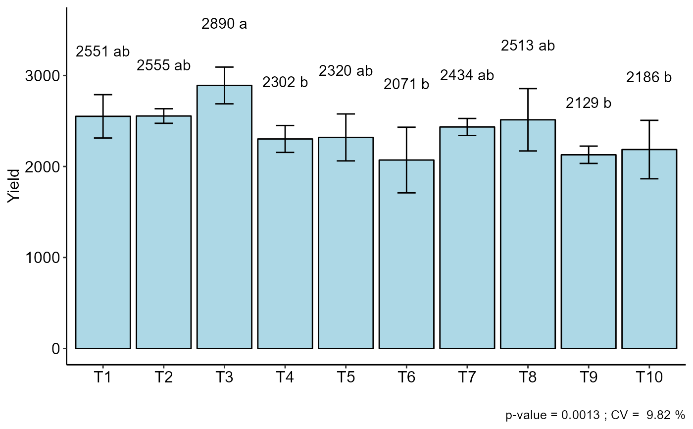 summarise_anova(list(a),design = "DBC")
#> | Yield |
#> T1 | 2551.25 ab |
#> T2 | 2554.75 ab |
#> T3 | 2890.5 a |
#> T4 | 2302.5 b |
#> T5 | 2319.5 ab |
#> T6 | 2071 b |
#> T7 | 2434.25 ab |
#> T8 | 2513.25 ab |
#> T9 | 2128.75 b |
#> T10 | 2186.25 b |
#> CV(%) | 9.821 |
#> p_tr | 0.001 |
#> p_bl | 0.354 |
#> Transformation | No transf |
#=====================================
# FAT2DIC
#=====================================
data(corn)
attach(corn)
#> The following objects are masked from covercrops (pos = 8):
#>
#> A, B, Resp
#> The following objects are masked from covercrops (pos = 10):
#>
#> A, B, Resp
a=FAT2DIC(A, B, Resp, quali=c(TRUE, TRUE))
#>
#> -----------------------------------------------------------------
#> Normality of errors
#> -----------------------------------------------------------------
#> Method Statistic p.value
#> Shapiro-Wilk normality test(W) 0.9704679 0.6785543
#>
#> As the calculated p-value is greater than the 5% significance level, hypothesis H0 is not rejected. Therefore, errors can be considered normal
#>
#> -----------------------------------------------------------------
#> Homogeneity of Variances
#> -----------------------------------------------------------------
#> Method Statistic p.value
#> Bartlett test(Bartlett's K-squared) 3.948702 0.5568251
#>
#> As the calculated p-value is greater than the 5% significance level, hypothesis H0 is not rejected. Therefore, the variances can be considered homogeneous
#>
#> -----------------------------------------------------------------
#> Independence from errors
#> -----------------------------------------------------------------
#> Method Statistic p.value
#> Durbin-Watson test(DW) 2.820109 0.8709071
#>
#> As the calculated p-value is greater than the 5% significance level, hypothesis H0 is not rejected. Therefore, errors can be considered independent
#>
#> -----------------------------------------------------------------
#> Additional Information
#> -----------------------------------------------------------------
#>
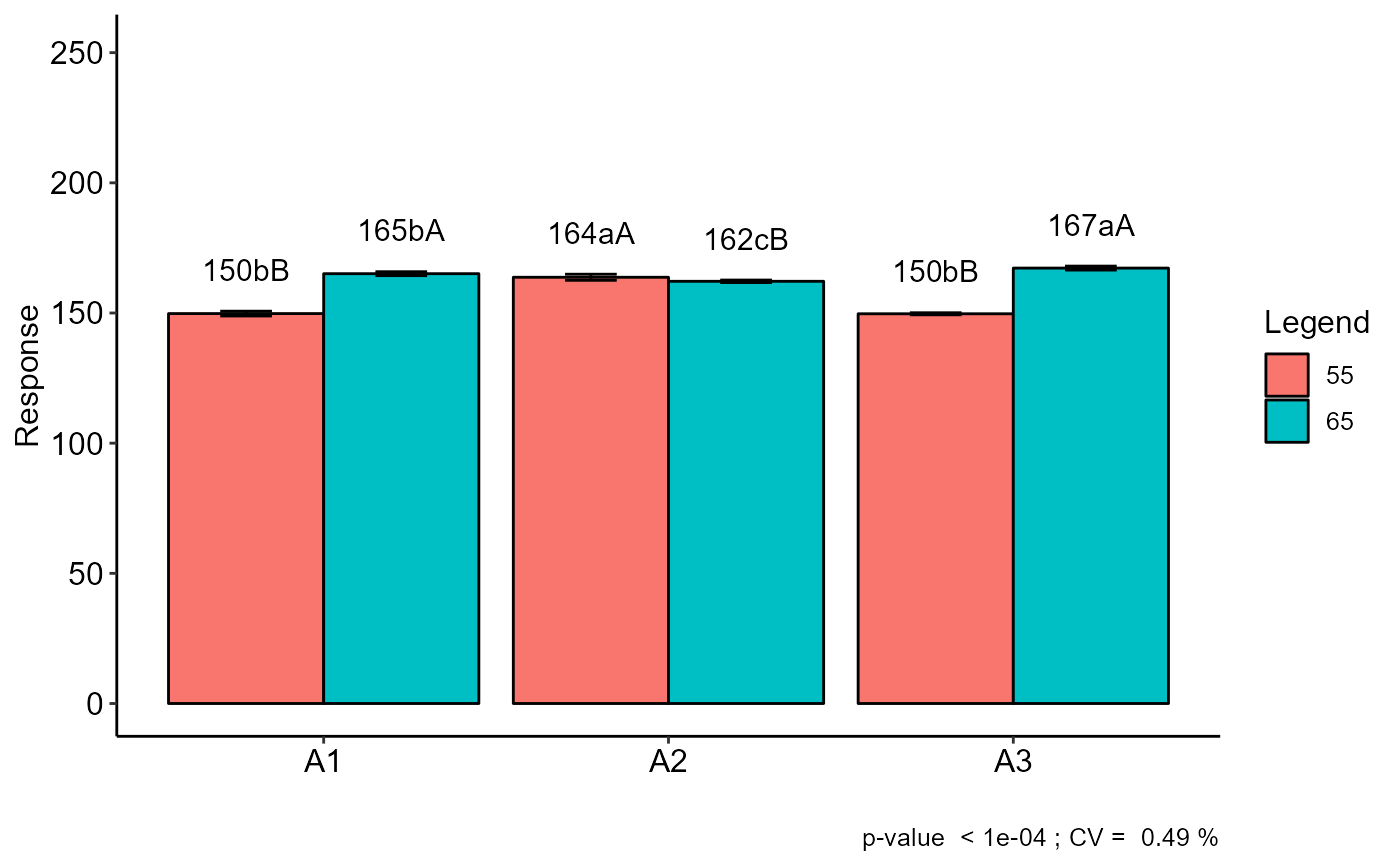
#> CV (%) = 0.49
#> Mean = 159.6208
#> Median = 162.55
#> Possible outliers = No discrepant point
#>
#> -----------------------------------------------------------------
#> Analysis of Variance
#> -----------------------------------------------------------------
#> Df Sum Sq Mean.Sq F value Pr(F)
#> Fator1 2 137.3058 68.6529167 110.0158 8.086134e-11
#> Fator2 1 654.1704 654.1704167 1048.3034 2.080297e-17
#> Fator1:Fator2 2 436.3508 218.1754167 349.6245 3.948414e-15
#> Residuals 18 11.2325 0.6240278
#>
#>
#> -----------------------------------------------------------------
#> Significant interaction: analyzing the interaction
#> -----------------------------------------------------------------
#>
#> -----------------------------------------------------------------
#> Analyzing F1 inside of each level of F2
#> -----------------------------------------------------------------
#>
#> Df Sum Sq Mean Sq F value Pr(>F)
#> Fator2 1 654.17 654.17 1048.303 < 2.2e-16 ***
#> Fator2:Fator1 4 573.66 143.41 229.820 3.492e-15 ***
#> Fator2:Fator1: 55 2 521.74 260.87 418.046 8.202e-16 ***
#> Fator2:Fator1: 65 2 51.91 25.96 41.594 1.784e-07 ***
#> Residuals 18 11.23 0.62
#> ---
#> Signif. codes: 0 '***' 0.001 '**' 0.01 '*' 0.05 '.' 0.1 ' ' 1
#>
#> -----------------------------------------------------------------
#> Analyzing F2 inside of the level of F1
#> -----------------------------------------------------------------
#>
#> Df Sum Sq Mean Sq F value Pr(>F)
#> Fator1 2 137.31 68.65 110.02 8.086e-11 ***
#> Fator1:Fator2 3 1090.52 363.51 582.52 < 2.2e-16 ***
#> Fator1:Fator2: A1 1 469.71 469.71 752.71 3.876e-16 ***
#> Fator1:Fator2: A2 1 4.81 4.81 7.70 0.01249 *
#> Fator1:Fator2: A3 1 616.00 616.00 987.14 < 2.2e-16 ***
#> Residuals 18 11.23 0.62
#> ---
#> Signif. codes: 0 '***' 0.001 '**' 0.01 '*' 0.05 '.' 0.1 ' ' 1
#>
#> -----------------------------------------------------------------
#> Final table
#> -----------------------------------------------------------------
#> 55 65
#> A1 150 bB 165 bA
#> A2 164 aA 162 cB
#> A3 150 bB 167 aA
#>
#>
#> Averages followed by the same lowercase letter in the column and
#> uppercase in the row do not differ by the tukey (p< 0.05 )
summarise_anova(list(a),design = "DBC")
#> | Yield |
#> T1 | 2551.25 ab |
#> T2 | 2554.75 ab |
#> T3 | 2890.5 a |
#> T4 | 2302.5 b |
#> T5 | 2319.5 ab |
#> T6 | 2071 b |
#> T7 | 2434.25 ab |
#> T8 | 2513.25 ab |
#> T9 | 2128.75 b |
#> T10 | 2186.25 b |
#> CV(%) | 9.821 |
#> p_tr | 0.001 |
#> p_bl | 0.354 |
#> Transformation | No transf |
#=====================================
# FAT2DIC
#=====================================
data(corn)
attach(corn)
#> The following objects are masked from covercrops (pos = 8):
#>
#> A, B, Resp
#> The following objects are masked from covercrops (pos = 10):
#>
#> A, B, Resp
a=FAT2DIC(A, B, Resp, quali=c(TRUE, TRUE))
#>
#> -----------------------------------------------------------------
#> Normality of errors
#> -----------------------------------------------------------------
#> Method Statistic p.value
#> Shapiro-Wilk normality test(W) 0.9704679 0.6785543
#>
#> As the calculated p-value is greater than the 5% significance level, hypothesis H0 is not rejected. Therefore, errors can be considered normal
#>
#> -----------------------------------------------------------------
#> Homogeneity of Variances
#> -----------------------------------------------------------------
#> Method Statistic p.value
#> Bartlett test(Bartlett's K-squared) 3.948702 0.5568251
#>
#> As the calculated p-value is greater than the 5% significance level, hypothesis H0 is not rejected. Therefore, the variances can be considered homogeneous
#>
#> -----------------------------------------------------------------
#> Independence from errors
#> -----------------------------------------------------------------
#> Method Statistic p.value
#> Durbin-Watson test(DW) 2.820109 0.8709071
#>
#> As the calculated p-value is greater than the 5% significance level, hypothesis H0 is not rejected. Therefore, errors can be considered independent
#>
#> -----------------------------------------------------------------
#> Additional Information
#> -----------------------------------------------------------------
#>
#> CV (%) = 0.49
#> Mean = 159.6208
#> Median = 162.55
#> Possible outliers = No discrepant point
#>
#> -----------------------------------------------------------------
#> Analysis of Variance
#> -----------------------------------------------------------------
#> Df Sum Sq Mean.Sq F value Pr(F)
#> Fator1 2 137.3058 68.6529167 110.0158 8.086134e-11
#> Fator2 1 654.1704 654.1704167 1048.3034 2.080297e-17
#> Fator1:Fator2 2 436.3508 218.1754167 349.6245 3.948414e-15
#> Residuals 18 11.2325 0.6240278
#>
#>
#> -----------------------------------------------------------------
#> Significant interaction: analyzing the interaction
#> -----------------------------------------------------------------
#>
#> -----------------------------------------------------------------
#> Analyzing F1 inside of each level of F2
#> -----------------------------------------------------------------
#>
#> Df Sum Sq Mean Sq F value Pr(>F)
#> Fator2 1 654.17 654.17 1048.303 < 2.2e-16 ***
#> Fator2:Fator1 4 573.66 143.41 229.820 3.492e-15 ***
#> Fator2:Fator1: 55 2 521.74 260.87 418.046 8.202e-16 ***
#> Fator2:Fator1: 65 2 51.91 25.96 41.594 1.784e-07 ***
#> Residuals 18 11.23 0.62
#> ---
#> Signif. codes: 0 '***' 0.001 '**' 0.01 '*' 0.05 '.' 0.1 ' ' 1
#>
#> -----------------------------------------------------------------
#> Analyzing F2 inside of the level of F1
#> -----------------------------------------------------------------
#>
#> Df Sum Sq Mean Sq F value Pr(>F)
#> Fator1 2 137.31 68.65 110.02 8.086e-11 ***
#> Fator1:Fator2 3 1090.52 363.51 582.52 < 2.2e-16 ***
#> Fator1:Fator2: A1 1 469.71 469.71 752.71 3.876e-16 ***
#> Fator1:Fator2: A2 1 4.81 4.81 7.70 0.01249 *
#> Fator1:Fator2: A3 1 616.00 616.00 987.14 < 2.2e-16 ***
#> Residuals 18 11.23 0.62
#> ---
#> Signif. codes: 0 '***' 0.001 '**' 0.01 '*' 0.05 '.' 0.1 ' ' 1
#>
#> -----------------------------------------------------------------
#> Final table
#> -----------------------------------------------------------------
#> 55 65
#> A1 150 bB 165 bA
#> A2 164 aA 162 cB
#> A3 150 bB 167 aA
#>
#>
#> Averages followed by the same lowercase letter in the column and
#> uppercase in the row do not differ by the tukey (p< 0.05 )
 summarise_anova(list(a),design="FAT2DIC")
#> | Response |
#> A1 | - |
#> A2 | - |
#> A3 | - |
#> 55 | - |
#> 65 | - |
#> A1 55 | 150bB |
#> A1 65 | 165bA |
#> A2 55 | 164aA |
#> A2 65 | 162cB |
#> A3 55 | 150bB |
#> A3 65 | 167aA |
#> CV(%) | 0.495 |
#> p_F1 | p<0.001 |
#> p_F2 | p<0.001 |
#> p_F1xF2 | p<0.001 |
#> Transformation | No transf |
summarise_anova(list(a),design="FAT2DIC")
#> | Response |
#> A1 | - |
#> A2 | - |
#> A3 | - |
#> 55 | - |
#> 65 | - |
#> A1 55 | 150bB |
#> A1 65 | 165bA |
#> A2 55 | 164aA |
#> A2 65 | 162cB |
#> A3 55 | 150bB |
#> A3 65 | 167aA |
#> CV(%) | 0.495 |
#> p_F1 | p<0.001 |
#> p_F2 | p<0.001 |
#> p_F1xF2 | p<0.001 |
#> Transformation | No transf |