Analysis: Joint analysis of experiments in randomized block design in scheme factorial double
conjfat2dbc.RdFunction of the AgroR package for joint analysis of experiments conducted in a randomized factorial double in block design with balanced data. The function generates the joint analysis through two models. Model 1: F-test of the effects of Factor 1, Factor 2 and F1 x F2 interaction are used in reference to the mean square of the interaction with the year. Model 2: F-test of the Factor 1, Factor 2 and F1 x F2 interaction effects are used in reference to the mean square of the residual.
conjfat2dbc(
  f1,
  f2,
  block,
  experiment,
  response,
  transf = 1,
  constant = 0,
  model = 1,
  norm = "sw",
  homog = "bt",
  homog.value = 7,
  alpha.f = 0.05,
  alpha.t = 0.05
)
Arguments
- f1
Numeric or complex vector with factor 1 levels
- f2
Numeric or complex vector with factor 2 levels
- block
Numerical or complex vector with blocks
- experiment
Numeric or complex vector with locations or times
- response
Numerical vector containing the response of the experiment.
- transf
Applies data transformation (default is 1; for log consider 0)
- constant
Add a constant for transformation (enter value)
- model
Define model of the analysis of variance
- norm
Error normality test (default is Shapiro-Wilk)
- homog
Homogeneity test of variances (default is Bartlett)
- homog.value
Reference value for homogeneity of experiments. By default, this ratio should not be greater than 7
- alpha.f
Level of significance of the F test (default is 0.05)
- alpha.t
Significance level of the multiple comparison test (default is 0.05)
Value
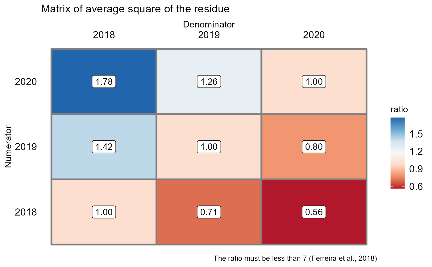
Returns the assumptions of the analysis of variance, the assumption of the joint analysis by means of a QMres ratio matrix and analysis of variance
Note
The function is still limited to analysis of variance and assumptions only.
References
Ferreira, P. V. Estatistica experimental aplicada a agronomia. Edufal, 2018.
Principles and procedures of statistics a biometrical approach Steel, Torry and Dickey. Third Edition 1997
Multiple comparisons theory and methods. Departament of statistics the Ohio State University. USA, 1996. Jason C. Hsu. Chapman Hall/CRC.
Practical Nonparametrics Statistics. W.J. Conover, 1999
Ramalho M.A.P., Ferreira D.F., Oliveira A.C. 2000. Experimentacao em Genetica e Melhoramento de Plantas. Editora UFLA.
Examples
library(AgroR)
ano=factor(rep(c(2018,2019,2020),e=48))
f1=rep(rep(c("A","B","C"),e=16),3)
f2=rep(rep(rep(c("a1","a2","a3","a4"),e=4),3),3)
resp=rnorm(48*3,10,1)
bloco=rep(c("b1","b2","b3","b4"),36)
dados=data.frame(ano,f1,f2,resp,bloco)
with(dados,conjfat2dbc(f1,f2,bloco,ano,resp, model=1))
#>
#> -----------------------------------------------------------------
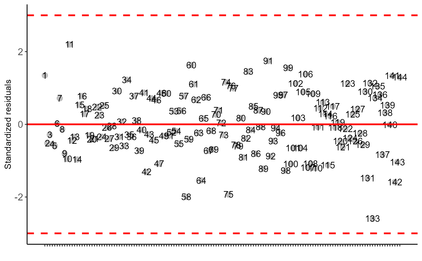
#> Normality of errors
#> -----------------------------------------------------------------
#> Method Statistic p.value
#> Shapiro-Wilk normality test(W) 0.9936686 0.7794519
#>
#> As the calculated p-value is greater than the 5% significance level, hypothesis H0 is not rejected. Therefore, errors can be considered normal
#> -----------------------------------------------------------------
#> Homogeneity of Variances
#> -----------------------------------------------------------------
#> Method Statistic p.value
#> Bartlett test(Bartlett's K-squared) 23.44848 0.0152697
#>
#> As the calculated p-value is less than the 5% significance level, H0 is rejected. Therefore, the variances are not homogeneous
#>
#> -----------------------------------------------------------------
#> Independence from errors
#> -----------------------------------------------------------------
#> Method Statistic p.value
#> Durbin-Watson test(DW) 2.568423 0.8143241
#>
#> As the calculated p-value is greater than the 5% significance level, hypothesis H0 is not rejected. Therefore, errors can be considered independent
#> -----------------------------------------------------------------
#> Test Homogeneity of experiments
#> -----------------------------------------------------------------
#> [1] 1.779032
#>
#> Based on the analysis of variance and homogeneity of experiments, it can be concluded that:
#> The experiments can be analyzed together
 #>
#>
#>
#>
 #>
#> -----------------------------------------------------------------
#> Analysis of variance
#> -----------------------------------------------------------------
#> Df Sum Sq Mean Sq F value Pr(>F)
#> f1 2 1.588736 0.7943681 0.6529516 0.5303031
#> f2 3 8.457173 2.8190575 2.3171980 0.1035156
#> f1:f2 6 8.344925 1.3908208 1.1432215 0.3710006
#> local:bloco 11 12.026048 1.0932771 0.8986477 0.5563127
#> f1:f2:local 22 26.764767 1.2165803 1.2587297 0.1270165
#> Residuals 99 95.684923 0.9665144
#>
#> -----------------------------------------------------------------
#>
#>
#> -----------------------------------------------------------------
#> Analysis of variance
#> -----------------------------------------------------------------
#> Df Sum Sq Mean Sq F value Pr(>F)
#> f1 2 1.588736 0.7943681 0.6529516 0.5303031
#> f2 3 8.457173 2.8190575 2.3171980 0.1035156
#> f1:f2 6 8.344925 1.3908208 1.1432215 0.3710006
#> local:bloco 11 12.026048 1.0932771 0.8986477 0.5563127
#> f1:f2:local 22 26.764767 1.2165803 1.2587297 0.1270165
#> Residuals 99 95.684923 0.9665144
#>
#> -----------------------------------------------------------------
#>