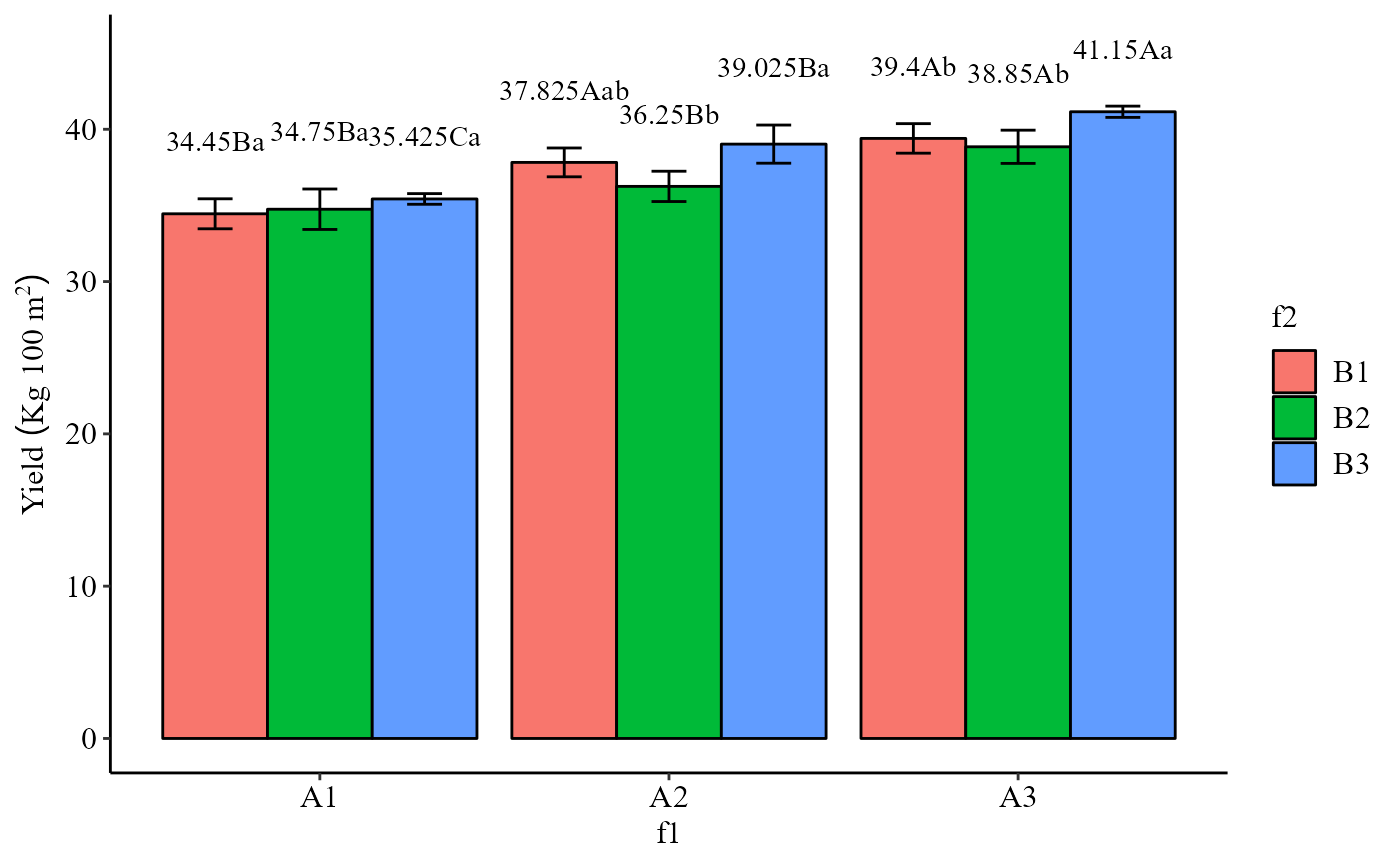
Graph: Invert letters for two factor chart
ibarplot.double.Rdinvert uppercase and lowercase letters in graph for factorial scheme the subdivided plot with significant interaction
ibarplot.double(analysis)Arguments
- analysis
FAT2DIC, FAT2DBC, PSUBDIC or PSUBDBC object
Value
Return column chart for two factors
Examples
data(covercrops)
attach(covercrops)
#> The following objects are masked from covercrops (pos = 4):
#>
#> A, B, Bloco, Resp
a=FAT2DBC(A, B, Bloco, Resp, ylab=expression("Yield"~(Kg~"100 m"^2)),
legend = "Cover crops",alpha.f = 0.3,family = "serif")
#>
#> -----------------------------------------------------------------
#> Normality of errors
#> -----------------------------------------------------------------
#> Method Statistic p.value
#> Shapiro-Wilk normality test(W) 0.9758908 0.6061712
#>
#> As the calculated p-value is greater than the 5% significance level, hypothesis H0 is not rejected. Therefore, errors can be considered normal
#>
#> -----------------------------------------------------------------
#> Homogeneity of Variances
#> -----------------------------------------------------------------
#> Method Statistic p.value
#> Bartlett test(Bartlett's K-squared) 10.19232 0.2517862
#>
#> As the calculated p-value is greater than the 5% significance level, hypothesis H0 is not rejected. Therefore, the variances can be considered homogeneous
#>
#> -----------------------------------------------------------------
#> Independence from errors
#> -----------------------------------------------------------------
#> Method Statistic p.value
#> Durbin-Watson test(DW) 2.335214 0.3781148
#>
#> As the calculated p-value is greater than the 5% significance level, hypothesis H0 is not rejected. Therefore, errors can be considered independent
#>
#> -----------------------------------------------------------------
#> Additional Information
#> -----------------------------------------------------------------
#>
#> CV (%) = 2.65
#> Mean = 37.4583
#> Median = 37.45
#> Possible outliers = No discrepant point
#>
#> -----------------------------------------------------------------
#> Analysis of Variance
#> -----------------------------------------------------------------
#> Df Sum Sq Mean.Sq F value Pr(F)
#> Fator1 2 146.585000 73.292500 74.645449 4.979960e-11
#> Fator2 2 23.021667 11.510833 11.723318 2.805884e-04
#> bloco 3 2.167500 0.722500 0.735837 5.409183e-01
#> Fator1:Fator2 4 6.008333 1.502083 1.529811 2.252749e-01
#> Residuals 24 23.565000 0.981875
#>
#> -----------------------------------------------------------------
#>
#> Significant interaction: analyzing the interaction
#>
#> -----------------------------------------------------------------
#>
#> -----------------------------------------------------------------
#> Analyzing F1 inside of each level of F2
#> -----------------------------------------------------------------
#> Df Sum Sq Mean Sq F value Pr(>F)
#> bloco 3 2.168 0.723 0.7358 0.5409183
#> Fator2 2 23.022 11.511 11.7233 0.0002806 ***
#> Fator2:Fator1 6 152.593 25.432 25.9017 2.296e-09 ***
#> Fator2:Fator1: B1 2 51.165 25.583 26.0547 9.667e-07 ***
#> Fator2:Fator1: B2 2 34.427 17.213 17.5311 2.027e-05 ***
#> Fator2:Fator1: B3 2 67.002 33.501 34.1192 9.629e-08 ***
#> Residuals 24 23.565 0.982
#> ---
#> Signif. codes: 0 '***' 0.001 '**' 0.01 '*' 0.05 '.' 0.1 ' ' 1
#>
#> -----------------------------------------------------------------
#> Analyzing F2 inside of the level of F1
#> -----------------------------------------------------------------
#>
#> Df Sum Sq Mean Sq F value Pr(>F)
#> bloco 3 2.168 0.723 0.7358 0.540918
#> Fator1 2 146.585 73.293 74.6454 4.98e-11 ***
#> Fator1:Fator2 6 29.030 4.838 4.9276 0.002054 **
#> Fator1:Fator2: A1 2 1.995 0.998 1.0159 0.377120
#> Fator1:Fator2: A2 2 15.495 7.748 7.8905 0.002325 **
#> Fator1:Fator2: A3 2 11.540 5.770 5.8765 0.008371 **
#> Residuals 24 23.565 0.982
#> ---
#> Signif. codes: 0 '***' 0.001 '**' 0.01 '*' 0.05 '.' 0.1 ' ' 1
#>
#> -----------------------------------------------------------------
#> Final table
#> -----------------------------------------------------------------
#> B1 B2 B3
#> A1 34.5 bA 34.8 bA 35.4 cA
#> A2 37.8 aAB 36.2 bB 39.0 bA
#> A3 39.4 aB 38.9 aB 41.1 aA
#>
#>
#> Averages followed by the same lowercase letter in the column
#> and uppercase in the row do not differ by the tukey (p< 0.05 )
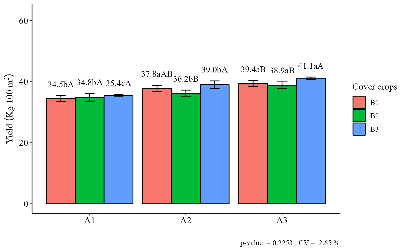 ibarplot.double(a)