Graph: Group FAT2DIC, FAT2DBC, PSUBDIC or PSUBDBC functions column charts
bargraph_twofactor.RdGroups two or more column charts exported from FAT2DIC, FAT2DBC, PSUBDIC or PSUBDBC function
bargraph_twofactor(
  analysis,
  labels = NULL,
  ocult.facet = FALSE,
  ocult.box = FALSE,
  facet.size = 14,
  ylab = NULL,
  width.bar = 0.3,
  sup = NULL
)
Arguments
- analysis
List with DIC, DBC or DQL object
- labels
Vector with the name of the facets
- ocult.facet
Hide facets
- ocult.box
Hide box
- facet.size
Font size facets
- ylab
Y-axis name
- width.bar
Width bar
- sup
Number of units above the standard deviation or average bar on the graph
Value
Returns a column chart grouped by facets
Examples
library(AgroR)
data(corn)
a=with(corn, FAT2DIC(A, B, Resp, quali=c(TRUE, TRUE),ylab="Heigth (cm)"))
#>
#> -----------------------------------------------------------------
#> Normality of errors
#> -----------------------------------------------------------------
#> Method Statistic p.value
#> Shapiro-Wilk normality test(W) 0.9704679 0.6785543
#>
#> As the calculated p-value is greater than the 5% significance level, hypothesis H0 is not rejected. Therefore, errors can be considered normal
#>
#> -----------------------------------------------------------------
#> Homogeneity of Variances
#> -----------------------------------------------------------------
#> Method Statistic p.value
#> Bartlett test(Bartlett's K-squared) 3.948702 0.5568251
#>
#> As the calculated p-value is greater than the 5% significance level, hypothesis H0 is not rejected. Therefore, the variances can be considered homogeneous
#>
#> -----------------------------------------------------------------
#> Independence from errors
#> -----------------------------------------------------------------
#> Method Statistic p.value
#> Durbin-Watson test(DW) 2.820109 0.8709071
#>
#> As the calculated p-value is greater than the 5% significance level, hypothesis H0 is not rejected. Therefore, errors can be considered independent
#>
#> -----------------------------------------------------------------
#> Additional Information
#> -----------------------------------------------------------------
#>
#> CV (%) = 0.49
#> Mean = 159.6208
#> Median = 162.55
#> Possible outliers = No discrepant point
#>
#> -----------------------------------------------------------------
#> Analysis of Variance
#> -----------------------------------------------------------------
#> Df Sum Sq Mean.Sq F value Pr(F)
#> Fator1 2 137.3058 68.6529167 110.0158 8.086134e-11
#> Fator2 1 654.1704 654.1704167 1048.3034 2.080297e-17
#> Fator1:Fator2 2 436.3508 218.1754167 349.6245 3.948414e-15
#> Residuals 18 11.2325 0.6240278
#>
#>
#> -----------------------------------------------------------------
#> Significant interaction: analyzing the interaction
#> -----------------------------------------------------------------
#>
#> -----------------------------------------------------------------
#> Analyzing F1 inside of each level of F2
#> -----------------------------------------------------------------
#>
#> Df Sum Sq Mean Sq F value Pr(>F)
#> Fator2 1 654.17 654.17 1048.303 < 2.2e-16 ***
#> Fator2:Fator1 4 573.66 143.41 229.820 3.492e-15 ***
#> Fator2:Fator1: 55 2 521.74 260.87 418.046 8.202e-16 ***
#> Fator2:Fator1: 65 2 51.91 25.96 41.594 1.784e-07 ***
#> Residuals 18 11.23 0.62
#> ---
#> Signif. codes: 0 '***' 0.001 '**' 0.01 '*' 0.05 '.' 0.1 ' ' 1
#>
#> -----------------------------------------------------------------
#> Analyzing F2 inside of the level of F1
#> -----------------------------------------------------------------
#>
#> Df Sum Sq Mean Sq F value Pr(>F)
#> Fator1 2 137.31 68.65 110.02 8.086e-11 ***
#> Fator1:Fator2 3 1090.52 363.51 582.52 < 2.2e-16 ***
#> Fator1:Fator2: A1 1 469.71 469.71 752.71 3.876e-16 ***
#> Fator1:Fator2: A2 1 4.81 4.81 7.70 0.01249 *
#> Fator1:Fator2: A3 1 616.00 616.00 987.14 < 2.2e-16 ***
#> Residuals 18 11.23 0.62
#> ---
#> Signif. codes: 0 '***' 0.001 '**' 0.01 '*' 0.05 '.' 0.1 ' ' 1
#>
#> -----------------------------------------------------------------
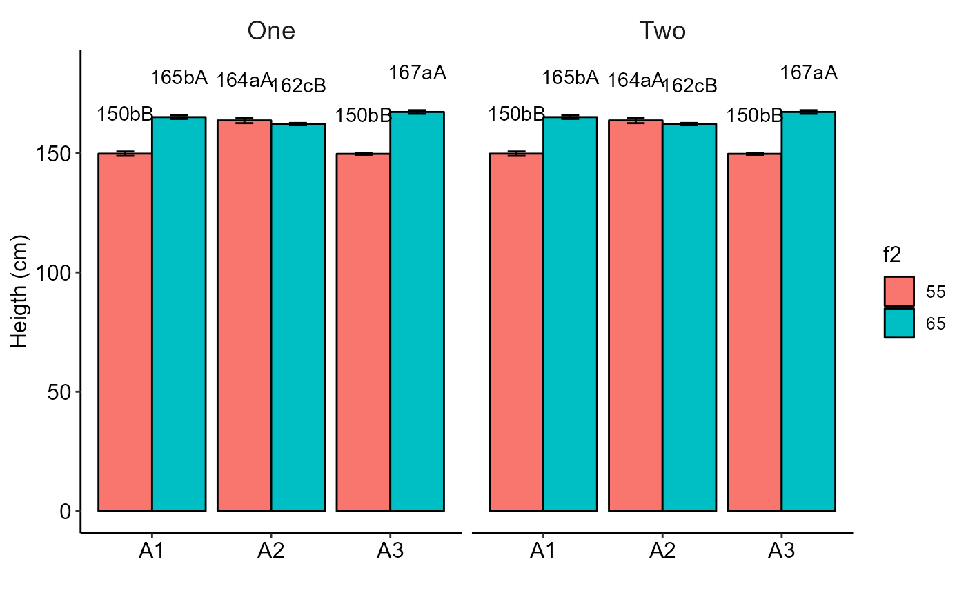
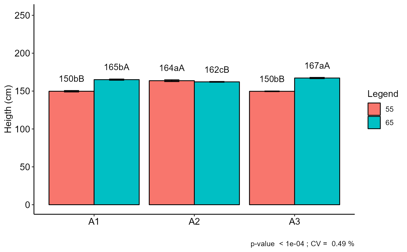
#> Final table
#> -----------------------------------------------------------------
#> 55 65
#> A1 150 bB 165 bA
#> A2 164 aA 162 cB
#> A3 150 bB 167 aA
#>
#>
#> Averages followed by the same lowercase letter in the column and
#> uppercase in the row do not differ by the tukey (p< 0.05 )
 b=with(corn, FAT2DIC(A, B, Resp, mcomp="sk", quali=c(TRUE, TRUE),ylab="Heigth (cm)"))
#>
#> -----------------------------------------------------------------
#> Normality of errors
#> -----------------------------------------------------------------
#> Method Statistic p.value
#> Shapiro-Wilk normality test(W) 0.9704679 0.6785543
#>
#> As the calculated p-value is greater than the 5% significance level, hypothesis H0 is not rejected. Therefore, errors can be considered normal
#>
#> -----------------------------------------------------------------
#> Homogeneity of Variances
#> -----------------------------------------------------------------
#> Method Statistic p.value
#> Bartlett test(Bartlett's K-squared) 3.948702 0.5568251
#>
#> As the calculated p-value is greater than the 5% significance level, hypothesis H0 is not rejected. Therefore, the variances can be considered homogeneous
#>
#> -----------------------------------------------------------------
#> Independence from errors
#> -----------------------------------------------------------------
#> Method Statistic p.value
#> Durbin-Watson test(DW) 2.820109 0.8709071
#>
#> As the calculated p-value is greater than the 5% significance level, hypothesis H0 is not rejected. Therefore, errors can be considered independent
#>
#> -----------------------------------------------------------------
#> Additional Information
#> -----------------------------------------------------------------
#>
#> CV (%) = 0.49
#> Mean = 159.6208
#> Median = 162.55
#> Possible outliers = No discrepant point
#>
#> -----------------------------------------------------------------
#> Analysis of Variance
#> -----------------------------------------------------------------
#> Df Sum Sq Mean.Sq F value Pr(F)
#> Fator1 2 137.3058 68.6529167 110.0158 8.086134e-11
#> Fator2 1 654.1704 654.1704167 1048.3034 2.080297e-17
#> Fator1:Fator2 2 436.3508 218.1754167 349.6245 3.948414e-15
#> Residuals 18 11.2325 0.6240278
#>
#>
#> -----------------------------------------------------------------
#> Significant interaction: analyzing the interaction
#> -----------------------------------------------------------------
#>
#> -----------------------------------------------------------------
#> Analyzing F1 inside of each level of F2
#> -----------------------------------------------------------------
#>
#> Df Sum Sq Mean Sq F value Pr(>F)
#> Fator2 1 654.17 654.17 1048.303 < 2.2e-16 ***
#> Fator2:Fator1 4 573.66 143.41 229.820 3.492e-15 ***
#> Fator2:Fator1: 55 2 521.74 260.87 418.046 8.202e-16 ***
#> Fator2:Fator1: 65 2 51.91 25.96 41.594 1.784e-07 ***
#> Residuals 18 11.23 0.62
#> ---
#> Signif. codes: 0 '***' 0.001 '**' 0.01 '*' 0.05 '.' 0.1 ' ' 1
#>
#> -----------------------------------------------------------------
#> Analyzing F2 inside of the level of F1
#> -----------------------------------------------------------------
#>
#> Df Sum Sq Mean Sq F value Pr(>F)
#> Fator1 2 137.31 68.65 110.02 8.086e-11 ***
#> Fator1:Fator2 3 1090.52 363.51 582.52 < 2.2e-16 ***
#> Fator1:Fator2: A1 1 469.71 469.71 752.71 3.876e-16 ***
#> Fator1:Fator2: A2 1 4.81 4.81 7.70 0.01249 *
#> Fator1:Fator2: A3 1 616.00 616.00 987.14 < 2.2e-16 ***
#> Residuals 18 11.23 0.62
#> ---
#> Signif. codes: 0 '***' 0.001 '**' 0.01 '*' 0.05 '.' 0.1 ' ' 1
#>
#> -----------------------------------------------------------------
#> Final table
#> -----------------------------------------------------------------
#> 55 65
#> A1 150 bB 165 bA
#> A2 164 aA 162 cB
#> A3 150 bB 167 aA
#>
#>
#> Averages followed by the same lowercase letter in the column and
#> uppercase in the row do not differ by the sk (p< 0.05 )
b=with(corn, FAT2DIC(A, B, Resp, mcomp="sk", quali=c(TRUE, TRUE),ylab="Heigth (cm)"))
#>
#> -----------------------------------------------------------------
#> Normality of errors
#> -----------------------------------------------------------------
#> Method Statistic p.value
#> Shapiro-Wilk normality test(W) 0.9704679 0.6785543
#>
#> As the calculated p-value is greater than the 5% significance level, hypothesis H0 is not rejected. Therefore, errors can be considered normal
#>
#> -----------------------------------------------------------------
#> Homogeneity of Variances
#> -----------------------------------------------------------------
#> Method Statistic p.value
#> Bartlett test(Bartlett's K-squared) 3.948702 0.5568251
#>
#> As the calculated p-value is greater than the 5% significance level, hypothesis H0 is not rejected. Therefore, the variances can be considered homogeneous
#>
#> -----------------------------------------------------------------
#> Independence from errors
#> -----------------------------------------------------------------
#> Method Statistic p.value
#> Durbin-Watson test(DW) 2.820109 0.8709071
#>
#> As the calculated p-value is greater than the 5% significance level, hypothesis H0 is not rejected. Therefore, errors can be considered independent
#>
#> -----------------------------------------------------------------
#> Additional Information
#> -----------------------------------------------------------------
#>
#> CV (%) = 0.49
#> Mean = 159.6208
#> Median = 162.55
#> Possible outliers = No discrepant point
#>
#> -----------------------------------------------------------------
#> Analysis of Variance
#> -----------------------------------------------------------------
#> Df Sum Sq Mean.Sq F value Pr(F)
#> Fator1 2 137.3058 68.6529167 110.0158 8.086134e-11
#> Fator2 1 654.1704 654.1704167 1048.3034 2.080297e-17
#> Fator1:Fator2 2 436.3508 218.1754167 349.6245 3.948414e-15
#> Residuals 18 11.2325 0.6240278
#>
#>
#> -----------------------------------------------------------------
#> Significant interaction: analyzing the interaction
#> -----------------------------------------------------------------
#>
#> -----------------------------------------------------------------
#> Analyzing F1 inside of each level of F2
#> -----------------------------------------------------------------
#>
#> Df Sum Sq Mean Sq F value Pr(>F)
#> Fator2 1 654.17 654.17 1048.303 < 2.2e-16 ***
#> Fator2:Fator1 4 573.66 143.41 229.820 3.492e-15 ***
#> Fator2:Fator1: 55 2 521.74 260.87 418.046 8.202e-16 ***
#> Fator2:Fator1: 65 2 51.91 25.96 41.594 1.784e-07 ***
#> Residuals 18 11.23 0.62
#> ---
#> Signif. codes: 0 '***' 0.001 '**' 0.01 '*' 0.05 '.' 0.1 ' ' 1
#>
#> -----------------------------------------------------------------
#> Analyzing F2 inside of the level of F1
#> -----------------------------------------------------------------
#>
#> Df Sum Sq Mean Sq F value Pr(>F)
#> Fator1 2 137.31 68.65 110.02 8.086e-11 ***
#> Fator1:Fator2 3 1090.52 363.51 582.52 < 2.2e-16 ***
#> Fator1:Fator2: A1 1 469.71 469.71 752.71 3.876e-16 ***
#> Fator1:Fator2: A2 1 4.81 4.81 7.70 0.01249 *
#> Fator1:Fator2: A3 1 616.00 616.00 987.14 < 2.2e-16 ***
#> Residuals 18 11.23 0.62
#> ---
#> Signif. codes: 0 '***' 0.001 '**' 0.01 '*' 0.05 '.' 0.1 ' ' 1
#>
#> -----------------------------------------------------------------
#> Final table
#> -----------------------------------------------------------------
#> 55 65
#> A1 150 bB 165 bA
#> A2 164 aA 162 cB
#> A3 150 bB 167 aA
#>
#>
#> Averages followed by the same lowercase letter in the column and
#> uppercase in the row do not differ by the sk (p< 0.05 )
 bargraph_twofactor(analysis = list(a,b), labels = c("One","Two"),ocult.box = TRUE)