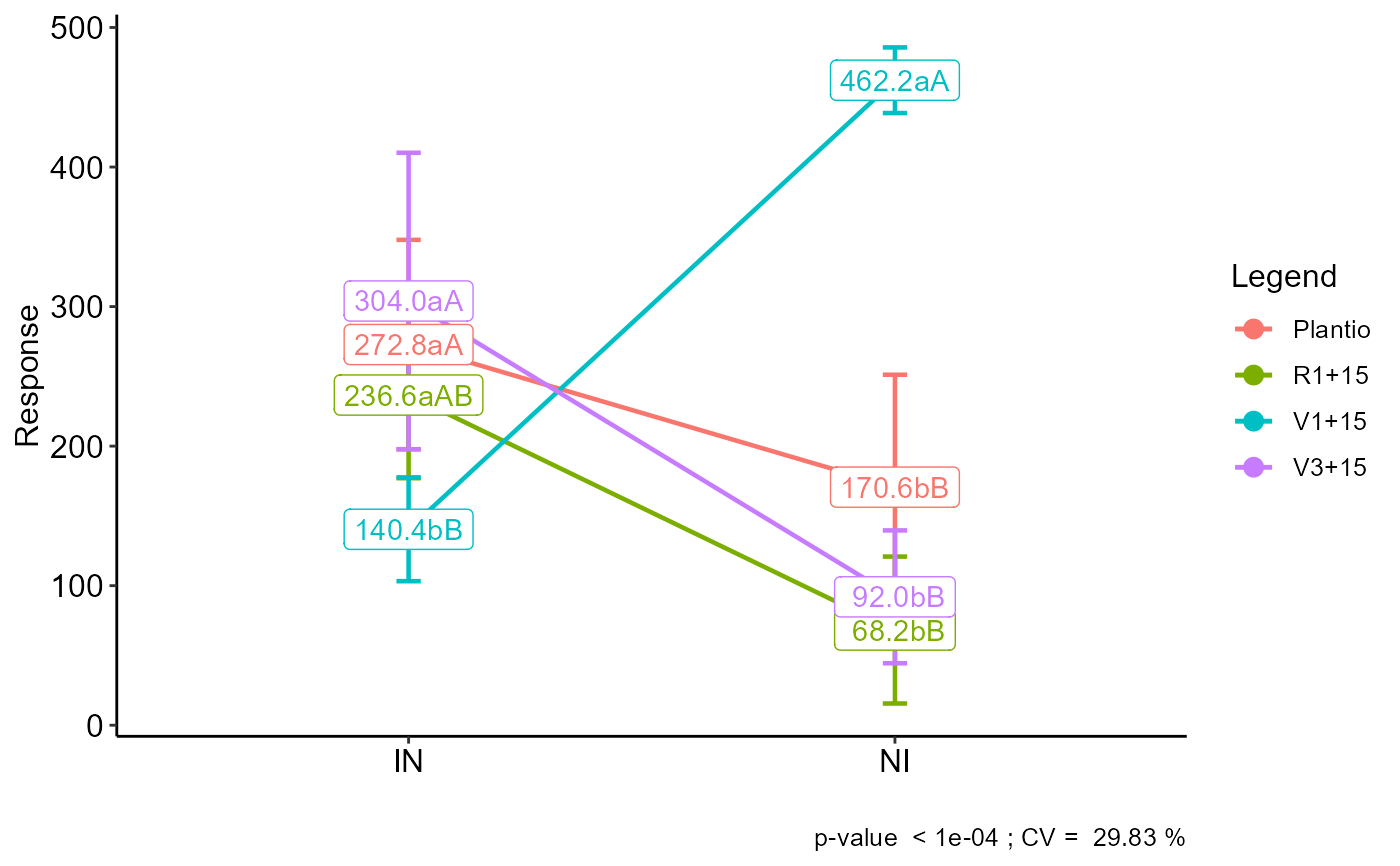
Graph: Interaction plot
plot_interaction.RdPerforms an interaction graph from an output of the FAT2DIC, FAT2DBC, PSUBDIC or PSUBDBC commands.
plot_interaction(
  a,
  box_label = TRUE,
  repel = FALSE,
  pointsize = 3,
  linesize = 0.8,
  width.bar = 0.05,
  add.errorbar = TRUE
)
Arguments
- a
FAT2DIC, FAT2DBC, PSUBDIC or PSUBDBC object
- box_label
Add box in label
- repel
a boolean, whether to use ggrepel to avoid overplotting text labels or not.
- pointsize
Point size
- linesize
Line size (Trendline and Error Bar)
- width.bar
width of the error bars.
- add.errorbar
Add error bars.
Value
Returns an interaction graph with averages and letters from the multiple comparison test
Examples
data(cloro)
a=with(cloro, FAT2DIC(f1, f2, resp))
#>
#> -----------------------------------------------------------------
#> Normality of errors
#> -----------------------------------------------------------------
#> Method Statistic p.value
#> Shapiro-Wilk normality test(W) 0.9680878 0.3125183
#>
#> As the calculated p-value is greater than the 5% significance level, hypothesis H0 is not rejected. Therefore, errors can be considered normal
#>
#> -----------------------------------------------------------------
#> Homogeneity of Variances
#> -----------------------------------------------------------------
#> Method Statistic p.value
#> Bartlett test(Bartlett's K-squared) 9.875441 0.1957427
#>
#> As the calculated p-value is greater than the 5% significance level, hypothesis H0 is not rejected. Therefore, the variances can be considered homogeneous
#>
#> -----------------------------------------------------------------
#> Independence from errors
#> -----------------------------------------------------------------
#> Method Statistic p.value
#> Durbin-Watson test(DW) 2.04374 0.1482695
#>
#> As the calculated p-value is greater than the 5% significance level, hypothesis H0 is not rejected. Therefore, errors can be considered independent
#>
#> -----------------------------------------------------------------
#> Additional Information
#> -----------------------------------------------------------------
#>
#> CV (%) = 29.83
#> Mean = 218.35
#> Median = 185
#> Possible outliers = No discrepant point
#>
#> -----------------------------------------------------------------
#> Analysis of Variance
#> -----------------------------------------------------------------
#> Df Sum Sq Mean.Sq F value Pr(F)
#> Fator1 1 16160.4 16160.4 3.810516 5.972867e-02
#> Fator2 3 116554.5 38851.5 9.160929 1.596453e-04
#> Fator1:Fator2 3 452096.2 150698.7 35.533773 2.663131e-10
#> Residuals 32 135712.0 4241.0
#>
#>
#> -----------------------------------------------------------------
#> Significant interaction: analyzing the interaction
#> -----------------------------------------------------------------
#>
#> -----------------------------------------------------------------
#> Analyzing F1 inside of each level of F2
#> -----------------------------------------------------------------
#>
#> Df Sum Sq Mean Sq F value Pr(>F)
#> Fator2 3 116554 38851 9.1609 0.0001596 ***
#> Fator2:Fator1 4 468257 117064 27.6030 5.661e-10 ***
#> Fator2:Fator1: Plantio 1 26112 26112 6.1571 0.0185315 *
#> Fator2:Fator1: R1+15 1 70896 70896 16.7169 0.0002728 ***
#> Fator2:Fator1: V1+15 1 258888 258888 61.0441 6.522e-09 ***
#> Fator2:Fator1: V3+15 1 112360 112360 26.4938 1.295e-05 ***
#> Residuals 32 135712 4241
#> ---
#> Signif. codes: 0 '***' 0.001 '**' 0.01 '*' 0.05 '.' 0.1 ' ' 1
#>
#> -----------------------------------------------------------------
#> Analyzing F2 inside of the level of F1
#> -----------------------------------------------------------------
#>
#> Df Sum Sq Mean Sq F value Pr(>F)
#> Fator1 1 16160 16160 3.8105 0.059729 .
#> Fator1:Fator2 6 568651 94775 22.3474 3.699e-10 ***
#> Fator1:Fator2: IN 3 75470 25157 5.9318 0.002454 **
#> Fator1:Fator2: NI 3 493181 164394 38.7629 9.117e-11 ***
#> Residuals 32 135712 4241
#> ---
#> Signif. codes: 0 '***' 0.001 '**' 0.01 '*' 0.05 '.' 0.1 ' ' 1
#>
#> -----------------------------------------------------------------
#> Final table
#> -----------------------------------------------------------------
#> Plantio R1+15 V1+15 V3+15
#> IN 272.8 aA 236.6 aAB 140.4 bB 304.0 aA
#> NI 170.6 bB 68.2 bB 462.2 aA 92.0 bB
#>
#>
#> Averages followed by the same lowercase letter in the column and
#> uppercase in the row do not differ by the tukey (p< 0.05 )
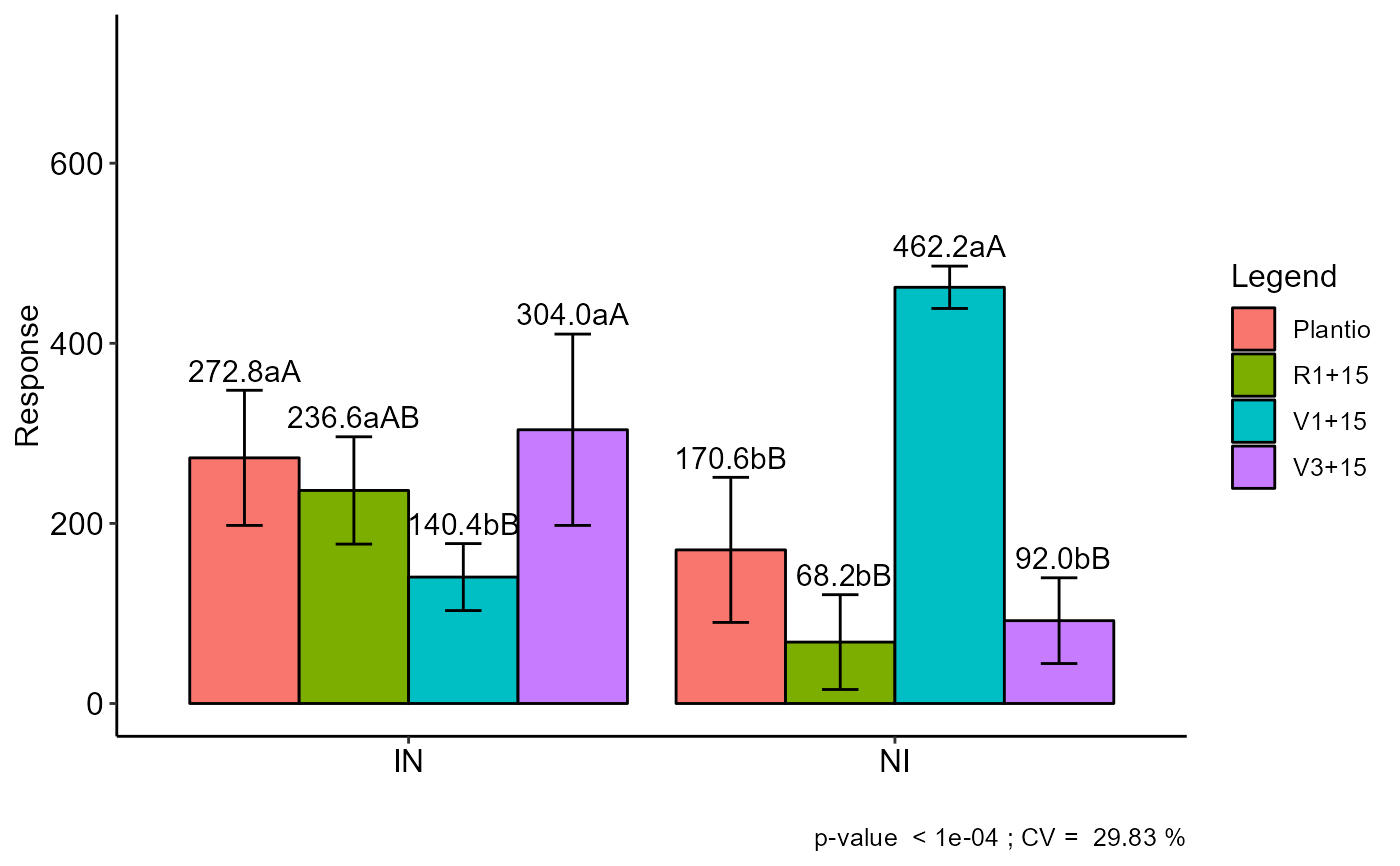 plot_interaction(a)