Analysis: Logistic regression — logistic • AgroR

Logistic regression is a very popular analysis in agrarian sciences, such as in fruit growth curves, seed germination, etc...The logistic function performs the analysis using 3 or 4 parameters of the logistic model, being imported from the LL function .3 or LL.4 of the drc package (Ritz & Ritz, 2016).

logistic(
  trat,
  resp,
  npar = "LL.3",
  error = "SE",
  ylab = "Dependent",
  xlab = expression("Independent"),
  theme = theme_classic(),
  legend.position = "top",
  r2 = "all",
  width.bar = NA,
  scale = "none",
  textsize = 12,
  font.family = "sans"
)

Arguments

trat: Numerical or complex vector with treatments
resp: Numerical vector containing the response of the experiment.
npar: Number of model parameters
error: Error bar (It can be SE - default, SD or FALSE)
ylab: Variable response name (Accepts the expression() function)
xlab: Treatments name (Accepts the expression() function)
theme: ggplot2 theme (default is theme_bw())
legend.position: Legend position (default is c(0.3,0.8))
r2: Coefficient of determination of the mean or all values (default is all)
width.bar: Bar width
scale: Sets x scale (default is none, can be "log")
textsize: Font size
font.family: Font family (default is sans)

Value

The function allows the automatic graph and equation construction of the logistic model, provides important statistics, such as the Akaike (AIC) and Bayesian (BIC) inference criteria, coefficient of determination (r2), square root of the mean error ( RMSE).

Details

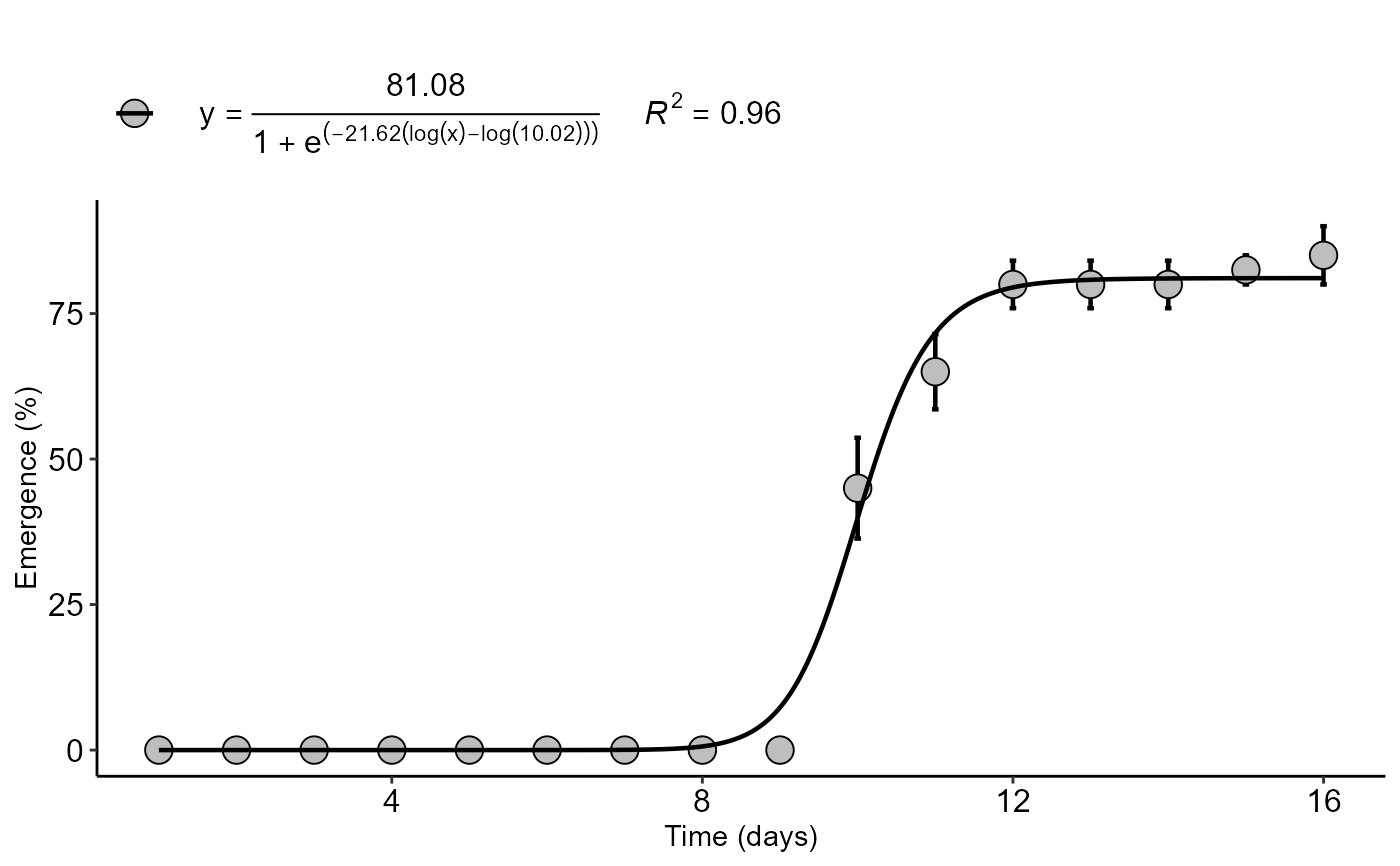
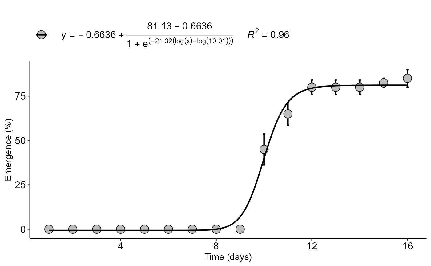
The three-parameter log-logistic function with lower limit 0 is $$f(x) = 0 + \frac{d}{1+\exp(b(\log(x)-\log(e)))}$$ The four-parameter log-logistic function is given by the expression $$f(x) = c + \frac{d-c}{1+\exp(b(\log(x)-\log(e)))}$$ The function is symmetric about the inflection point (e).

References

Seber, G. A. F. and Wild, C. J (1989) Nonlinear Regression, New York: Wiley and Sons (p. 330).

Ritz, C.; Strebig, J.C.; Ritz, M.C. Package ‘drc’. Creative Commons: Mountain View, CA, USA, 2016.

Author

Model imported from the drc package (Ritz et al., 2016)

Gabriel Danilo Shimizu

Leandro Simoes Azeredo Goncalves

Examples

data("emerg")
with(emerg, logistic(time, resp,xlab="Time (days)",ylab="Emergence (%)"))
#> $Coefficients
#>                Estimate  Std Error    t value      P-value   
#> b:(Intercept) -21.61550 3.56104842  -6.069982 8.912223e-08 **
#> d:(Intercept)  81.08478 1.73973123  46.607646 1.052258e-49 **
#> e:(Intercept)  10.01534 0.08344181 120.027785 1.852496e-74 **
#> 
#> $values
#>   Parameter     values
#> 1       AIC 434.790623
#> 2       BIC 443.426156
#> 3 r-squared   0.960000
#> 4      RMSE   6.789404
#> 
#> $graph

#> 
with(emerg, logistic(time, resp,npar="LL.4",xlab="Time (days)",ylab="Emergence (%)"))
#> $Coefficients
#>                Estimate  Std Error     t value      P-value   
#> b:(Intercept) -21.32060 3.53758836  -6.0268741 1.107976e-07 **
#> c:(Intercept)  -0.66355 1.22035166  -0.5437367 5.886374e-01 ns
#> d:(Intercept)  81.13072 1.75277913  46.2869040 5.929524e-49 **
#> e:(Intercept)  10.00733 0.08446958 118.4725590 3.826623e-73 **
#> 
#> $values
#>   Parameter     values
#> 1       AIC 436.475255
#> 2       BIC 447.269671
#> 3 r-squared   0.960000
#> 4      RMSE   6.772697
#> 
#> $graph

#>