Analysis: Completely randomized design with an additional treatment for quantitative factor
dic.ad.RdStatistical analysis of experiments conducted in a completely randomized with an additional treatment and balanced design with a factor considering the fixed model.
dic.ad(
  trat,
  response,
  responsead,
  grau = 1,
  norm = "sw",
  homog = "bt",
  alpha.f = 0.05,
  theme = theme_classic(),
  ylab = "response",
  xlab = "independent",
  family = "sans",
  posi = "top",
  pointsize = 4.5,
  linesize = 0.8,
  width.bar = NA,
  point = "mean_sd"
)
Arguments
- trat
Numerical or complex vector with treatments
- response
Numerical vector containing the response of the experiment.
- responsead
Numerical vector with additional treatment responses
- grau
Degree of polynomial in case of quantitative factor (default is 1)
- norm
Error normality test (default is Shapiro-Wilk)
- homog
Homogeneity test of variances (default is Bartlett)
- alpha.f
Level of significance of the F test (default is 0.05)
- theme
ggplot2 theme (default is theme_classic())
- ylab
Variable response name (Accepts the expression() function)
- xlab
Treatments name (Accepts the expression() function)
- family
Font family
- posi
Legend position
- pointsize
Point size
- linesize
line size (Trendline and Error Bar)
- width.bar
width of the error bars of a regression graph.
- point
Defines whether to plot mean ("mean"), mean with standard deviation ("mean_sd" - default) or mean with standard error (default - "mean_se"). For quali=FALSE or quali=TRUE.
Value
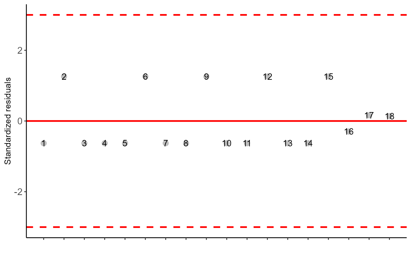
The table of analysis of variance, the test of normality of errors (Shapiro-Wilk ("sw"), Lilliefors ("li"), Anderson-Darling ("ad"), Cramer-von Mises ("cvm"), Pearson ("pearson") and Shapiro-Francia ("sf")), the test of homogeneity of variances (Bartlett ("bt") or Levene ("levene")), the test of independence of Durbin-Watson errors, adjustment of regression models up to grade 3 polynomial. The function also returns a standardized residual plot.
Note
In some experiments, the researcher may study a quantitative factor, such as fertilizer doses, and present a control, such as a reference fertilizer, treated as a qualitative control. In these cases, there is a difference between considering only the residue in the unfolding of the polynomial, removing or not the qualitative treatment, or since a treatment is excluded from the analysis. In this approach, the residue used is also considering the qualitative treatment, a method similar to the factorial scheme with additional control.
Examples
datadicad=data.frame(doses = c(rep(c(1:5),e=3)),
resp = c(3,4,3,5,5,6,7,7,8,4,4,5,2,2,3))
with(datadicad,dic.ad(doses, resp, rnorm(3,6,0.1),grau=2))
#>
#> -----------------------------------------------------------------
#> Normality of errors
#> -----------------------------------------------------------------
#> Method Statistic p.value
#> Shapiro-Wilk normality test(W) 0.68831 5.858208e-05
#>
#> As the calculated p-value is less than the 5% significance level, H0 is rejected. Therefore, errors do not follow a normal distribution
#>
#> -----------------------------------------------------------------
#> Homogeneity of Variances
#> -----------------------------------------------------------------
#> Method Statistic p.value
#> Bartlett test(Bartlett's K-squared) 3.099624 0.68463
#>
#> As the calculated p-value is greater than the 5% significance level,hypothesis H0 is not rejected. Therefore, the variances can be considered homogeneous
#>
#> -----------------------------------------------------------------
#> Independence from errors
#> -----------------------------------------------------------------
#> Method Statistic p.value
#> Durbin-Watson test(DW) 2.889275 0.80449
#>
#> As the calculated p-value is greater than the 5% significance level, hypothesis H0 is not rejected. Therefore, errors can be considered independent
 #>
#> -----------------------------------------------------------------
#> Additional Information
#> -----------------------------------------------------------------
#>
#> CV (%) = 11.69
#> Mean = 4.5333
#> Median = 4
#> Possible outliers = No discrepant point
#>
#> -----------------------------------------------------------------
#> Analysis of Variance
#> -----------------------------------------------------------------
#> Analysis of Variance Table
#>
#> Response: response
#> Df Sum Sq Mean Sq F value Pr(>F)
#> Factor 4 44.400 11.1000 39.516 8.118e-07 ***
#> Factor vs control 1 4.969 4.9686 17.688 0.001219 **
#> Residuals 12 3.371 0.2809
#> ---
#> Signif. codes: 0 '***' 0.001 '**' 0.01 '*' 0.05 '.' 0.1 ' ' 1
#>
#> ----------------------------------------------------
#> Regression Models
#> ----------------------------------------------------
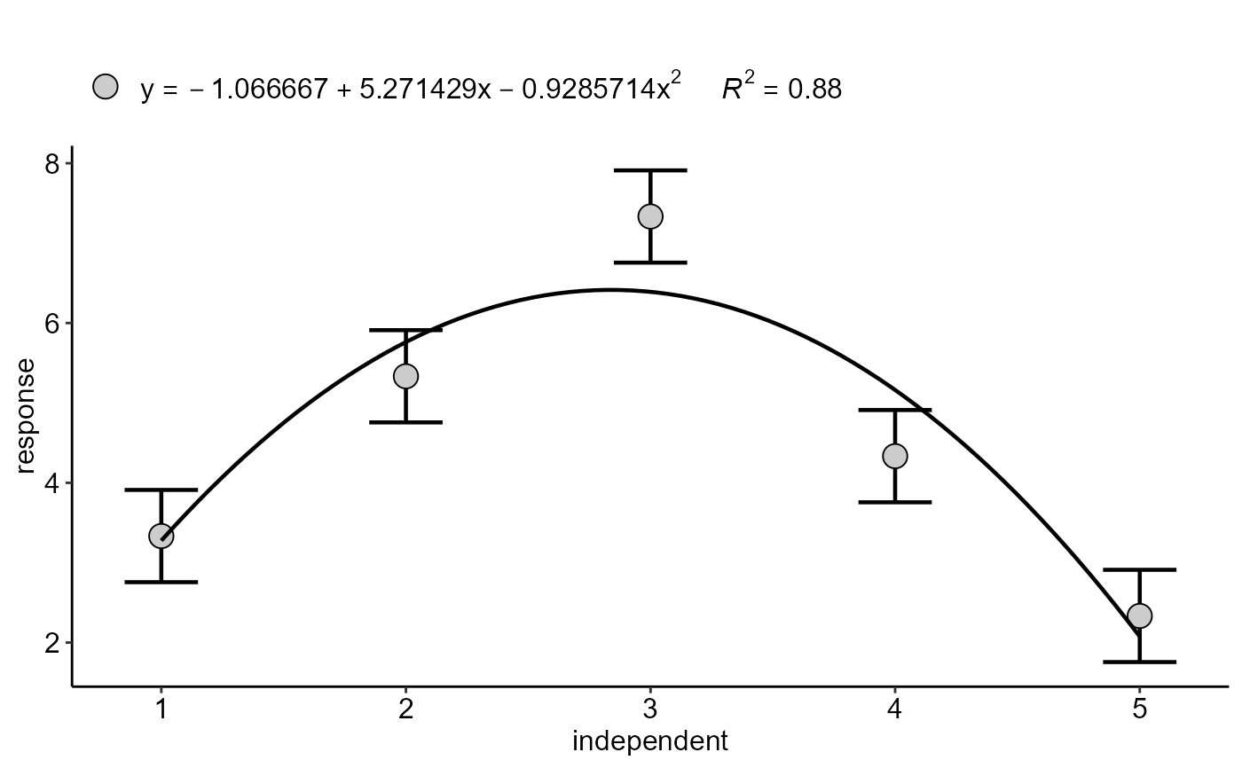
#> Estimate Std. Error t value Pr(>|t|)
#> (Intercept) -1.0666667 1.0615452 -1.004824 3.348137e-01
#> trat 5.2714286 0.8089681 6.516238 2.867473e-05
#> I(trat^2) -0.9285714 0.1322804 -7.019719 1.395317e-05
#>
#> ----------------------------------------------------
#> Deviations from regression
#> ----------------------------------------------------
#> Df SSq MSQ F p-value
#> Linear 1 2.700000 2.7000000 9.611869 9.184851e-03
#> Quadratic 1 36.214286 36.2142857 128.921099 8.933502e-08
#> Deviation 2 5.485714 2.7428571 9.764438 3.039740e-03
#> Residual 12 3.370832 0.2809027
#>
#> -----------------------------------------------------------------
#> Additional Information
#> -----------------------------------------------------------------
#>
#> CV (%) = 11.69
#> Mean = 4.5333
#> Median = 4
#> Possible outliers = No discrepant point
#>
#> -----------------------------------------------------------------
#> Analysis of Variance
#> -----------------------------------------------------------------
#> Analysis of Variance Table
#>
#> Response: response
#> Df Sum Sq Mean Sq F value Pr(>F)
#> Factor 4 44.400 11.1000 39.516 8.118e-07 ***
#> Factor vs control 1 4.969 4.9686 17.688 0.001219 **
#> Residuals 12 3.371 0.2809
#> ---
#> Signif. codes: 0 '***' 0.001 '**' 0.01 '*' 0.05 '.' 0.1 ' ' 1
#>
#> ----------------------------------------------------
#> Regression Models
#> ----------------------------------------------------
#> Estimate Std. Error t value Pr(>|t|)
#> (Intercept) -1.0666667 1.0615452 -1.004824 3.348137e-01
#> trat 5.2714286 0.8089681 6.516238 2.867473e-05
#> I(trat^2) -0.9285714 0.1322804 -7.019719 1.395317e-05
#>
#> ----------------------------------------------------
#> Deviations from regression
#> ----------------------------------------------------
#> Df SSq MSQ F p-value
#> Linear 1 2.700000 2.7000000 9.611869 9.184851e-03
#> Quadratic 1 36.214286 36.2142857 128.921099 8.933502e-08
#> Deviation 2 5.485714 2.7428571 9.764438 3.039740e-03
#> Residual 12 3.370832 0.2809027