Analysis: DIC experiments in split-plot
PSUBDIC.RdAnalysis of an experiment conducted in a completely randomized design in a split-plot scheme using fixed effects analysis of variance.
PSUBDIC(
  f1,
  f2,
  block,
  response,
  norm = "sw",
  alpha.f = 0.05,
  alpha.t = 0.05,
  quali = c(TRUE, TRUE),
  mcomp = "tukey",
  grau = c(NA, NA),
  grau12 = NA,
  grau21 = NA,
  transf = 1,
  constant = 0,
  geom = "bar",
  theme = theme_classic(),
  ylab = "Response",
  xlab = "",
  xlab.factor = c("F1", "F2"),
  fill = "lightblue",
  angle = 0,
  family = "sans",
  color = "rainbow",
  legend = "Legend",
  errorbar = TRUE,
  addmean = TRUE,
  textsize = 12,
  labelsize = 4,
  dec = 3,
  ylim = NA,
  posi = "right",
  point = "mean_se",
  angle.label = 0
)
Arguments
- f1
Numeric or complex vector with plot levels
- f2
Numeric or complex vector with subplot levels
- block
Numeric or complex vector with blocks
- response
Numeric vector with responses
- norm
Error normality test (default is Shapiro-Wilk)
- alpha.f
Level of significance of the F test (default is 0.05)
- alpha.t
Significance level of the multiple comparison test (default is 0.05)
- quali
Defines whether the factor is quantitative or qualitative (qualitative)
- mcomp
Multiple comparison test (Tukey (default), LSD, Scott-Knott and Duncan)
- grau
Polynomial degree in case of quantitative factor (default is 1). Provide a vector with three elements.
- grau12
Polynomial degree in case of quantitative factor (default is 1). Provide a vector with n levels of factor 2, in the case of interaction f1 x f2 and qualitative factor 2 and quantitative factor 1.
- grau21
Polynomial degree in case of quantitative factor (default is 1). Provide a vector with n levels of factor 1, in the case of interaction f1 x f2 and qualitative factor 1 and quantitative factor 2.
- transf
Applies data transformation (default is 1; for log consider 0)
- constant
Add a constant for transformation (enter value)
- geom
Graph type (columns or segments (For simple effect only))
- theme
ggplot2 theme (default is theme_classic())
- ylab
Variable response name (Accepts the expression() function)
- xlab
Treatments name (Accepts the expression() function)
- xlab.factor
Provide a vector with two observations referring to the x-axis name of factors 1 and 2, respectively, when there is an isolated effect of the factors. This argument uses `parse`.
- fill
Defines chart color (to generate different colors for different treatments, define fill = "trat")
- angle
x-axis scale text rotation
- family
Font family (default is sans)
- color
When the columns are different colors (Set fill-in argument as "trat")
- legend
Legend title name
- errorbar
Plot the standard deviation bar on the graph (In the case of a segment and column graph) - default is TRUE
- addmean
Plot the average value on the graph (default is TRUE)
- textsize
Font size (default is 12)
- labelsize
Label size (default is 4)
- dec
Number of cells (default is 3)
- ylim
y-axis limit
- posi
Legend position
- point
This function defines whether the point must have all points ("all"), mean ("mean"), standard deviation (default - "mean_sd") or mean with standard error ("mean_se") if quali= FALSE. For quali=TRUE, `mean_sd` and `mean_se` change which information will be displayed in the error bar.
- angle.label
Label angle
Value
The table of analysis of variance, the test of normality of errors (Shapiro-Wilk, Lilliefors, Anderson-Darling, Cramer-von Mises, Pearson and Shapiro-Francia), the test of homogeneity of variances (Bartlett), the test of multiple comparisons (Tukey, LSD, Scott-Knott or Duncan) or adjustment of regression models up to grade 3 polynomial, in the case of quantitative treatments. The column chart for qualitative treatments is also returned. The function also returns a standardized residual plot.
Note
The order of the chart follows the alphabetical pattern. Please use `scale_x_discrete` from package ggplot2, `limits` argument to reorder x-axis. The bars of the column and segment graphs are standard deviation.
In the final output when transformation (transf argument) is different from 1, the columns resp and respo in the mean test are returned, indicating transformed and non-transformed mean, respectively.
References
Principles and procedures of statistics a biometrical approach Steel, Torry and Dickey. Third Edition 1997
Multiple comparisons theory and methods. Departament of statistics the Ohio State University. USA, 1996. Jason C. Hsu. Chapman Hall/CRC.
Practical Nonparametrics Statistics. W.J. Conover, 1999
Ramalho M.A.P., Ferreira D.F., Oliveira A.C. 2000. Experimentacao em Genetica e Melhoramento de Plantas. Editora UFLA.
Scott R.J., Knott M. 1974. A cluster analysis method for grouping mans in the analysis of variance. Biometrics, 30, 507-512.
Examples
#===================================
# Example tomate
#===================================
# Obs. Consider that the "tomato" experiment is a completely randomized design.
library(AgroR)
data(tomate)
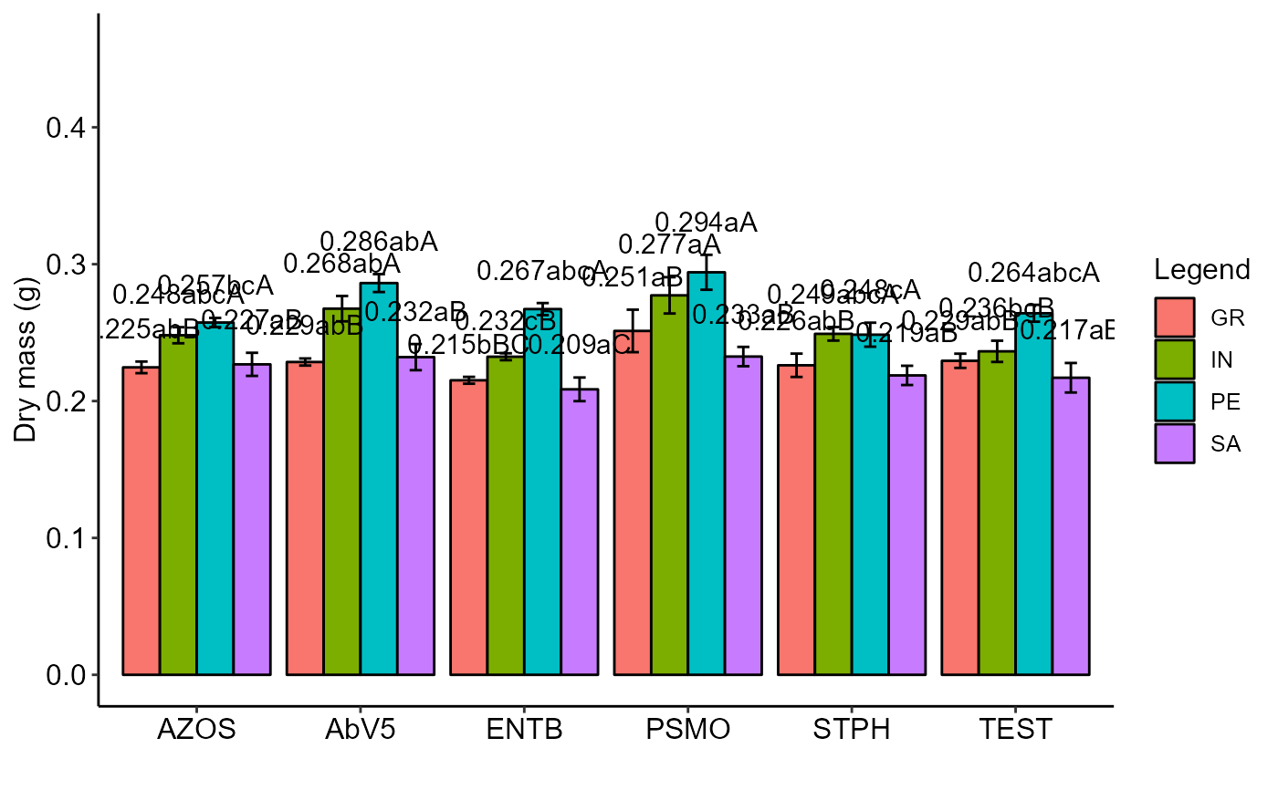
with(tomate, PSUBDIC(parc, subp, bloco, resp, ylab="Dry mass (g)"))
#> boundary (singular) fit: see help('isSingular')
#>
#> -----------------------------------------------------------------
#> Normality of errors
#> -----------------------------------------------------------------
#> Method Statistic p.value
#> Shapiro-Wilk normality test(W) 0.9636318 0.009177611
#>
#> As the calculated p-value is less than the 5% significance level, H0 is rejected. Therefore, errors do not follow a normal distribution
#>
#>
#> -----------------------------------------------------------------
#> Homogeneity of Variances
#> -----------------------------------------------------------------
#> Plot
#> Method Statistic p.value
#> Bartlett test(Bartlett's K-squared) 6.761137 0.2390196
#>
#> As the calculated p-value is greater than the 5% significance level, hypothesis H0 is not rejected. Therefore, the variances can be considered homogeneous
#>
#> ----------------------------------------------------
#> Split-plot
#> Method Statistic p.value
#> Bartlett test(Bartlett's K-squared) 5.451767 0.1415521
#>
#> As the calculated p-value is greater than the 5% significance level, hypothesis H0 is not rejected. Therefore, the variances can be considered homogeneous
#>
#> ----------------------------------------------------
#> Interaction
#> Method Statistic p.value
#> Bartlett test(Bartlett's K-squared) 34.15961 0.0628852
#>
#> As the calculated p-value is greater than the 5% significance level, hypothesis H0 is not rejected. Therefore, the variances can be considered homogeneous
#>
#> -----------------------------------------------------------------
#> Additional Information
#> -----------------------------------------------------------------
#>
#> CV1 (%) = 10.67
#> CV2 (%) = 4.55
#> Mean = 0.2433
#> Median = 0.2402
#>
#>
#> -----------------------------------------------------------------
#> Analysis of Variance
#> -----------------------------------------------------------------
#> Df Sum Sq Mean Sq F value Pr(>F)
#> F1 5 0.012779159 0.0025558319 3.793889 0.016
#> Error A 18 0.012126072 0.0006736707
#> F2 3 0.033333572 0.0111111908 90.570262 p<0.001
#> F1 x F2 15 0.004012849 0.0002675233 2.180653 0.019
#> Error B 54 0.006624738 0.0001226803
#>
#>
#> Your analysis is not valid, suggests using a try to transform the data
#>
#>
#> -----------------------------------------------------------------
#> Significant interaction: analyzing the interaction
#> -----------------------------------------------------------------
#> Analyzing F1 inside of each level of F2
#> -----------------------------------------------------------------
#> GL SQ QM Fc p.value
#> F1 : F2 GR 5.00000 0.00285200 0.000570 2.190341 0.074853
#> F1 : F2 IN 5.00000 0.00612400 0.001225 4.702737 0.001855
#> F1 : F2 PE 5.00000 0.00602100 0.001204 4.623975 0.00207
#> F1 : F2 SA 5.00000 0.00179500 0.000359 1.378652 0.253307
#> Combined error 39.14545 0.01017782 0.000260
#>
#> -----------------------------------------------------------------
#> Analyzing F2 inside of the level of F1
#> -----------------------------------------------------------------
#> GL SQ QM Fc p.value
#> F2 : F1 AZOS 3 0.003100 0.001033 8.422958 0.00011
#> F2 : F1 AbV5 3 0.009387 0.003129 25.506107 0
#> F2 : F1 ENTB 3 0.008261 0.002754 22.446718 0
#> F2 : F1 PSMO 3 0.008936 0.002979 24.280165 0
#> F2 : F1 STPH 3 0.002889 0.000963 7.850077 0.000194
#> F2 : F1 TEST 3 0.004773 0.001591 12.967502 2e-06
#> Error b 54 0.006625 0.000123
#>
#> -----------------------------------------------------------------
#> Final table
#> -----------------------------------------------------------------
#> GR IN PE SA
#> AZOS 0.225 abB 0.248 abcA 0.257 bcA 0.227 aB
#> AbV5 0.229 abB 0.268 abA 0.286 abA 0.232 aB
#> ENTB 0.215 bBC 0.232 cB 0.267 abcA 0.209 aC
#> PSMO 0.251 aB 0.277 aA 0.294 aA 0.233 aB
#> STPH 0.226 abB 0.249 abcA 0.248 cA 0.219 aB
#> TEST 0.229 abB 0.236 bcB 0.264 abcA 0.217 aB
#>
#>
#> Averages followed by the same lowercase letter in the column and uppercase in the row do not differ by the tukey (p< 0.05 )