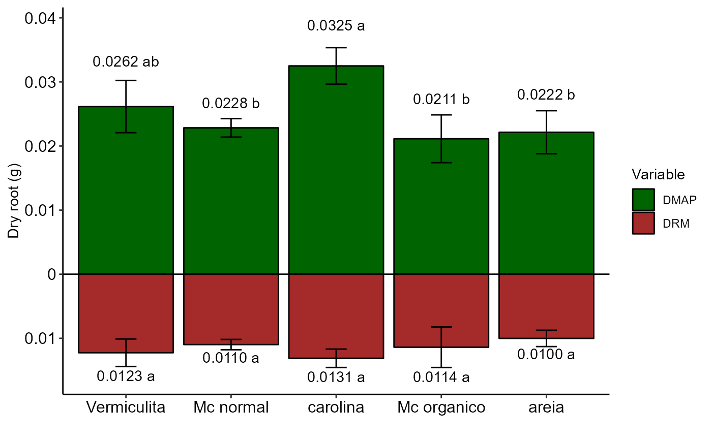
Graph: Positive barplot
barplot_positive.RdColumn chart with two variables that assume a positive response and represented by opposite sides, such as dry mass of the area and dry mass of the root
Arguments
- a
Object of DIC, DBC or DQL functions
- b
Object of DIC, DBC or DQL functions
- ylab
Y axis names
- var_name
Name of the variable
- legend.title
Legend title
- fill_color
Bar fill color
Value
The function returns a column chart with two positive sides
Note
When there is only an effect of the isolated factor in the case of factorial or subdivided plots, it is possible to use the barplot_positive function.
See also
Examples
data("passiflora")
attach(passiflora)
a=with(passiflora, DBC(trat, bloco, MSPA))
#>
#> -----------------------------------------------------------------
#> Normality of errors
#> -----------------------------------------------------------------
#> Method Statistic p.value
#> Shapiro-Wilk normality test(W) 0.9429864 0.2728826
#>
#> As the calculated p-value is greater than the 5% significance level, hypothesis H0 is not rejected. Therefore, errors can be considered normal
#>
#> -----------------------------------------------------------------
#> Homogeneity of Variances
#> -----------------------------------------------------------------
#> Method Statistic p.value
#> Bartlett test(Bartlett's K-squared) 4.070401 0.396562
#>
#> As the calculated p-value is greater than the 5% significance level, hypothesis H0 is not rejected. Therefore, the variances can be considered homogeneous
#>
#> -----------------------------------------------------------------
#> Independence from errors
#> -----------------------------------------------------------------
#> Method Statistic p.value
#> Durbin-Watson test(DW) 1.572708 0.03849032
#>
#> As the calculated p-value is less than the 5% significance level, H0 is rejected. Therefore, errors are not independent
#>
#> -----------------------------------------------------------------
#> Additional Information
#> -----------------------------------------------------------------
#>
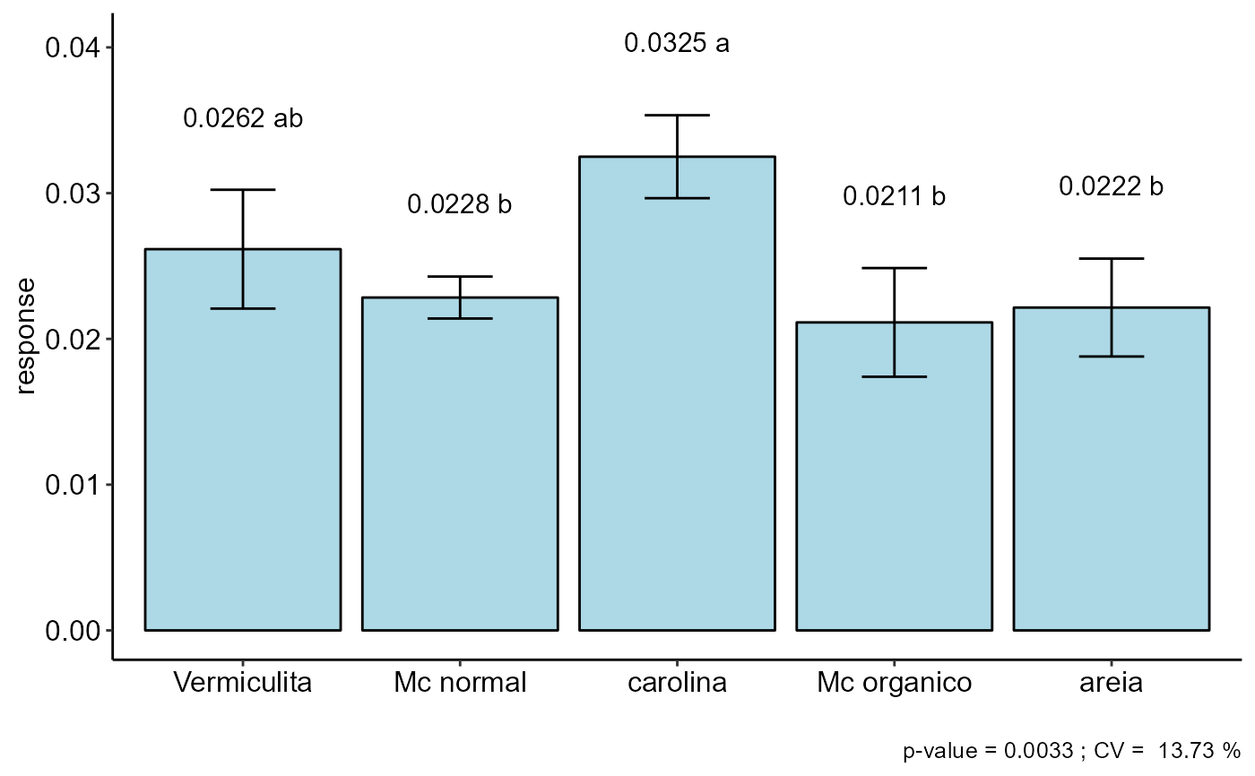
#> CV (%) = 13.73
#> MStrat/MST = 0.84
#> Mean = 0.025
#> Median = 0.0241
#> Possible outliers = No discrepant point
#>
#> -----------------------------------------------------------------
#> Analysis of Variance
#> -----------------------------------------------------------------
#> Df Sum Sq Mean.Sq F value Pr(F)
#> trat 4 3.413717e-04 8.534292e-05 7.2705205 0.003259252
#> bloco 3 1.506425e-05 5.021417e-06 0.4277837 0.736759950
#> Residuals 12 1.408586e-04 1.173821e-05
#>
#> As the calculated p-value, it is less than the 5% significance level. The hypothesis H0 of equality of means is rejected. Therefore, at least two treatments differ
#>
#> -----------------------------------------------------------------
#> Multiple Comparison Test: Tukey HSD
#> -----------------------------------------------------------------
#> resp groups
#> carolina 0.03250000 a
#> Vermiculita 0.02615625 ab
#> Mc normal 0.02283750 b
#> areia 0.02215000 b
#> Mc organico 0.02113125 b
#>
#>
#> Your analysis is not valid, suggests using a non-parametric
#> test and try to transform the data
 b=with(passiflora, DBC(trat, bloco, MSR))
#>
#> -----------------------------------------------------------------
#> Normality of errors
#> -----------------------------------------------------------------
#> Method Statistic p.value
#> Shapiro-Wilk normality test(W) 0.9836814 0.9723826
#>
#> As the calculated p-value is greater than the 5% significance level, hypothesis H0 is not rejected. Therefore, errors can be considered normal
#>
#> -----------------------------------------------------------------
#> Homogeneity of Variances
#> -----------------------------------------------------------------
#> Method Statistic p.value
#> Bartlett test(Bartlett's K-squared) 8.452343 0.076345
#>
#> As the calculated p-value is greater than the 5% significance level, hypothesis H0 is not rejected. Therefore, the variances can be considered homogeneous
#>
#> -----------------------------------------------------------------
#> Independence from errors
#> -----------------------------------------------------------------
#> Method Statistic p.value
#> Durbin-Watson test(DW) 1.826611 0.1152517
#>
#> As the calculated p-value is greater than the 5% significance level, hypothesis H0 is not rejected. Therefore, errors can be considered independent
#>
#> -----------------------------------------------------------------
#> Additional Information
#> -----------------------------------------------------------------
#>
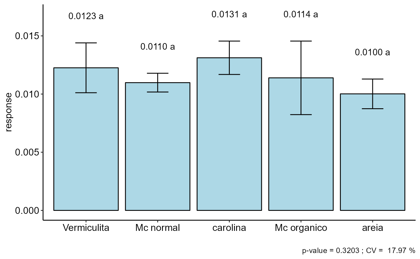
#> CV (%) = 17.97
#> MStrat/MST = 0.49
#> Mean = 0.0116
#> Median = 0.0112
#> Possible outliers = No discrepant point
#>
#> -----------------------------------------------------------------
#> Analysis of Variance
#> -----------------------------------------------------------------
#> Df Sum Sq Mean.Sq F value Pr(F)
#> trat 4 2.263485e-05 5.658712e-06 1.3123500 0.3203367
#> bloco 3 4.997083e-06 1.665694e-06 0.3863024 0.7648958
#> Residuals 12 5.174271e-05 4.311892e-06
#>
#> As the calculated p-value is greater than the 5% significance level, H0 is not rejected
b=with(passiflora, DBC(trat, bloco, MSR))
#>
#> -----------------------------------------------------------------
#> Normality of errors
#> -----------------------------------------------------------------
#> Method Statistic p.value
#> Shapiro-Wilk normality test(W) 0.9836814 0.9723826
#>
#> As the calculated p-value is greater than the 5% significance level, hypothesis H0 is not rejected. Therefore, errors can be considered normal
#>
#> -----------------------------------------------------------------
#> Homogeneity of Variances
#> -----------------------------------------------------------------
#> Method Statistic p.value
#> Bartlett test(Bartlett's K-squared) 8.452343 0.076345
#>
#> As the calculated p-value is greater than the 5% significance level, hypothesis H0 is not rejected. Therefore, the variances can be considered homogeneous
#>
#> -----------------------------------------------------------------
#> Independence from errors
#> -----------------------------------------------------------------
#> Method Statistic p.value
#> Durbin-Watson test(DW) 1.826611 0.1152517
#>
#> As the calculated p-value is greater than the 5% significance level, hypothesis H0 is not rejected. Therefore, errors can be considered independent
#>
#> -----------------------------------------------------------------
#> Additional Information
#> -----------------------------------------------------------------
#>
#> CV (%) = 17.97
#> MStrat/MST = 0.49
#> Mean = 0.0116
#> Median = 0.0112
#> Possible outliers = No discrepant point
#>
#> -----------------------------------------------------------------
#> Analysis of Variance
#> -----------------------------------------------------------------
#> Df Sum Sq Mean.Sq F value Pr(F)
#> trat 4 2.263485e-05 5.658712e-06 1.3123500 0.3203367
#> bloco 3 4.997083e-06 1.665694e-06 0.3863024 0.7648958
#> Residuals 12 5.174271e-05 4.311892e-06
#>
#> As the calculated p-value is greater than the 5% significance level, H0 is not rejected
 #>
#> -----------------------------------------------------------------
#> Multiple Comparison Test: Tukey HSD
#> -----------------------------------------------------------------
#> [1] "H0 is not rejected"
#>
#>
#> -----------------------------------------------------------------
#> Multiple Comparison Test: Tukey HSD
#> -----------------------------------------------------------------
#> [1] "H0 is not rejected"
#>
 barplot_positive(a, b, var_name = c("DMAP","DRM"), ylab = "Dry root (g)")