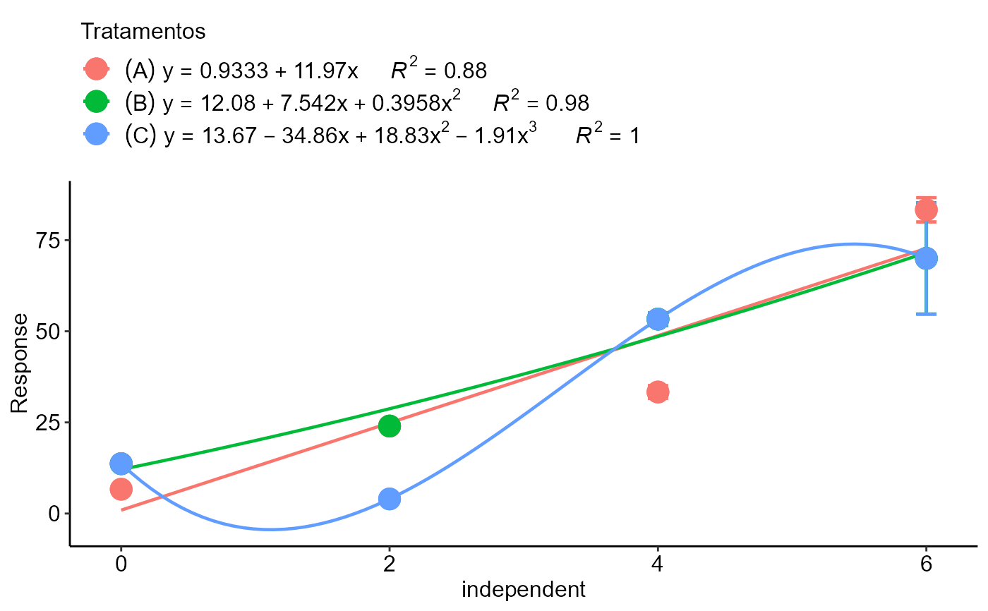
Analysis: Linear regression graph in double factorial with color graph
polynomial2_color.RdLinear regression analysis for significant interaction of an experiment with two factors, one quantitative and one qualitative
polynomial2_color(
  fator1,
  resp,
  fator2,
  color = NA,
  grau = NA,
  ylab = "Response",
  xlab = "independent",
  theme = theme_classic(),
  se = FALSE,
  point = "mean_se",
  legend.title = "Tratamentos",
  posi = "top",
  textsize = 12,
  ylim = NA,
  family = "sans",
  width.bar = NA,
  pointsize = 5,
  linesize = 0.8,
  separate = c("(\"", "\")"),
  n = NA,
  DFres = NA,
  SSq = NA
)
Arguments
- fator1
Numeric or complex vector with factor 1 levels
- resp
Numerical vector containing the response of the experiment.
- fator2
Numeric or complex vector with factor 2 levels
- color
Graph color (default is NA)
- grau
Degree of the polynomial (1,2 or 3)
- ylab
Dependent variable name (Accepts the expression() function)
- xlab
Independent variable name (Accepts the expression() function)
- theme
ggplot2 theme (default is theme_classic())
- se
Adds confidence interval (default is FALSE)
- point
Defines whether to plot all points ("all"), mean ("mean"), mean with standard deviation ("mean_sd") or mean with standard error (default - "mean_se").
- legend.title
Title legend
- posi
Legend position
- textsize
Font size (default is 12)
- ylim
y-axis scale
- family
Font family (default is sans)
- width.bar
width of the error bars of a regression graph.
- pointsize
Point size (default is 4)
- linesize
line size (Trendline and Error Bar)
- separate
Separation between treatment and equation (default is c("(\"","\")"))
- n
Number of decimal places for regression equations
- DFres
Residue freedom degrees
- SSq
Sum of squares of the residue
Value
Returns two or more linear, quadratic or cubic regression analyzes.
See also
Examples
dose=rep(c(0,0,0,2,2,2,4,4,4,6,6,6),3)
resp=c(8,7,5,23,24,25,30,34,36,80,90,80,
12,14,15,23,24,25,50,54,56,80,90,40,
12,14,15,3,4,5,50,54,56,80,90,40)
trat=rep(c("A","B","C"),e=12)
polynomial2_color(dose, resp, trat, grau=c(1,2,3))
#> Warning: NaNs produced
#>
#> ----------------------------------------------------
#> Regression Models
#> ----------------------------------------------------
#> $A
#>               Estimate Std. Error   t value     Pr(>|t|)
#> (Intercept)  0.9333333   5.395430 0.1729859 8.661137e-01
#> x           11.9666667   1.441989 8.2987205 8.528803e-06
#>
#> $B
#>               Estimate Std. Error   t value  Pr(>|t|)
#> (Intercept) 12.0833333  7.4460094 1.6227932 0.1390822
#> x            7.5416667  5.9788110 1.2613991 0.2388777
#> I(x^2)       0.3958333  0.9549306 0.4145153 0.6882023
#>
#> $C
#>               Estimate Std. Error   t value   Pr(>|t|)
#> (Intercept)  13.666667  7.7064187  1.773413 0.11409087
#> x           -34.861111 14.7845901 -2.357936 0.04610656
#> I(x^2)       18.833333  6.5334343  2.882609 0.02042957
#> I(x^3)       -1.909722  0.7180032 -2.659769 0.02881582
#>
#>
#> ----------------------------------------------------
#> Anova
#> ----------------------------------------------------
#> $`Anova A`
#>           Df      SSq       MSQ        F      p-value
#> Linear     1 8592.067 8592.0667 70.07576 1.401237e-08
#> Deviation  2 1155.600  577.8000  4.71246 1.877977e-02
#> Residual  24 2942.667  122.6111
#>
#> $`Anova B`
#>           Df        SSq        MSQ          F      p-value
#> Linear     1 5900.41667 5900.41667 48.1230177 3.571320e-07
#> Quadratic  1   30.08333   30.08333  0.2453557 6.248694e-01
#> Deviation  1  150.41667  150.41667  1.2267784 2.790120e-01
#> Residual  24 2942.66667  122.61111
#>
#> $`Anova C`
#>           Df          SSq       MSQ         F      p-value
#> Linear     1 7.150417e+03 7150.4167 58.317852 7.114165e-08
#> Quadratic  1 5.200833e+02  520.0833  4.241731 5.044762e-02
#> Cubic      1 1.260417e+03 1260.4167 10.279792 3.783350e-03
#> Deviation  0 4.547474e-13      -Inf      -Inf          NaN
#> Residual  24 2.942667e+03  122.6111
#>