Analysis: DBC experiments in double factorial
FAT2DBC.RdAnalysis of an experiment conducted in a randomized block design in a double factorial scheme using analysis of variance of fixed effects.
FAT2DBC(
  f1,
  f2,
  block,
  response,
  norm = "sw",
  homog = "bt",
  alpha.f = 0.05,
  alpha.t = 0.05,
  quali = c(TRUE, TRUE),
  mcomp = "tukey",
  grau = c(NA, NA),
  grau12 = NA,
  grau21 = NA,
  transf = 1,
  constant = 0,
  geom = "bar",
  theme = theme_classic(),
  ylab = "Response",
  xlab = "",
  xlab.factor = c("F1", "F2"),
  legend = "Legend",
  fill = "lightblue",
  angle = 0,
  textsize = 12,
  labelsize = 4,
  dec = 3,
  width.column = 0.9,
  width.bar = 0.3,
  family = "sans",
  point = "mean_sd",
  addmean = TRUE,
  errorbar = TRUE,
  CV = TRUE,
  sup = NA,
  color = "rainbow",
  posi = "right",
  ylim = NA,
  angle.label = 0
)
Arguments
- f1
Numeric or complex vector with factor 1 levels
- f2
Numeric or complex vector with factor 2 levels
- block
Numerical or complex vector with blocks
- response
Numerical vector containing the response of the experiment.
- norm
Error normality test (default is Shapiro-Wilk)
- homog
Homogeneity test of variances (default is Bartlett)
- alpha.f
Level of significance of the F test (default is 0.05)
- alpha.t
Significance level of the multiple comparison test (default is 0.05)
- quali
Defines whether the factor is quantitative or qualitative (qualitative)
- mcomp
Multiple comparison test (Tukey (default), LSD, Scott-Knott and Duncan)
- grau
Polynomial degree in case of quantitative factor (default is 1). Provide a vector with two elements.
- grau12
Polynomial degree in case of quantitative factor (default is 1). Provide a vector with n levels of factor 2, in the case of interaction f1 x f2 and qualitative factor 2 and quantitative factor 1.
- grau21
Polynomial degree in case of quantitative factor (default is 1). Provide a vector with n levels of factor 1, in the case of interaction f1 x f2 and qualitative factor 1 and quantitative factor 2.
- transf
Applies data transformation (default is 1; for log consider 0; `angular` for angular transformation)
- constant
Add a constant for transformation (enter value)
- geom
Graph type (columns or segments (For simple effect only))
- theme
ggplot2 theme (default is theme_classic())
- ylab
Variable response name (Accepts the expression() function)
- xlab
Treatments name (Accepts the expression() function)
- xlab.factor
Provide a vector with two observations referring to the x-axis name of factors 1 and 2, respectively, when there is an isolated effect of the factors. This argument uses `parse`.
- legend
Legend title name
- fill
Defines chart color (to generate different colors for different treatments, define fill = "trat")
- angle
x-axis scale text rotation
- textsize
font size
- labelsize
label size
- dec
number of cells
- width.column
Width column if geom="bar"
- width.bar
Width errorbar
- family
font family
- point
This function defines whether the point must have all points ("all"), mean ("mean"), standard deviation (default - "mean_sd") or mean with standard error ("mean_se") if quali= FALSE. For quali=TRUE, `mean_sd` and `mean_se` change which information will be displayed in the error bar.
- addmean
Plot the average value on the graph (default is TRUE)
- errorbar
Plot the standard deviation bar on the graph (In the case of a segment and column graph) - default is TRUE
- CV
Plotting the coefficient of variation and p-value of Anova (default is TRUE)
- sup
Number of units above the standard deviation or average bar on the graph
- color
Column chart color (default is "rainbow")
- posi
Legend position
- ylim
y-axis scale
- angle.label
label angle
Value
The table of analysis of variance, the test of normality of errors (Shapiro-Wilk, Lilliefors, Anderson-Darling, Cramer-von Mises, Pearson and Shapiro-Francia), the test of homogeneity of variances (Bartlett or Levene), the test of independence of Durbin-Watson errors, the test of multiple comparisons (Tukey, LSD, Scott-Knott or Duncan) or adjustment of regression models up to grade 3 polynomial, in the case of quantitative treatments. The column chart for qualitative treatments is also returned.
Note
The order of the chart follows the alphabetical pattern. Please use `scale_x_discrete` from package ggplot2, `limits` argument to reorder x-axis. The bars of the column and segment graphs are standard deviation.
The function does not perform multiple regression in the case of two quantitative factors.
In the final output when transformation (transf argument) is different from 1, the columns resp and respo in the mean test are returned, indicating transformed and non-transformed mean, respectively.
References
Principles and procedures of statistics a biometrical approach Steel, Torry and Dickey. Third Edition 1997
Multiple comparisons theory and methods. Departament of statistics the Ohio State University. USA, 1996. Jason C. Hsu. Chapman Hall/CRC.
Practical Nonparametrics Statistics. W.J. Conover, 1999
Ramalho M.A.P., Ferreira D.F., Oliveira A.C. 2000. Experimentacao em Genetica e Melhoramento de Plantas. Editora UFLA.
Scott R.J., Knott M. 1974. A cluster analysis method for grouping mans in the analysis of variance. Biometrics, 30, 507-512.
Mendiburu, F., and de Mendiburu, M. F. (2019). Package ‘agricolae’. R Package, Version, 1-2.
See also
Examples
#================================================
# Example cloro
#================================================
library(AgroR)
data(cloro)
attach(cloro)
#> The following objects are masked from cloro (pos = 3):
#>
#> bloco, f1, f2, resp
#> The following object is masked from simulate3:
#>
#> resp
#> The following object is masked from simulate1:
#>
#> resp
#> The following object is masked from aristolochia (pos = 6):
#>
#> resp
#> The following objects are masked from simulate2:
#>
#> bloco, resp
#> The following objects are masked from laranja:
#>
#> bloco, resp
#> The following object is masked from aristolochia (pos = 9):
#>
#> resp
#> The following objects are masked from cloro (pos = 10):
#>
#> bloco, f1, f2, resp
#> The following object is masked from passiflora:
#>
#> bloco
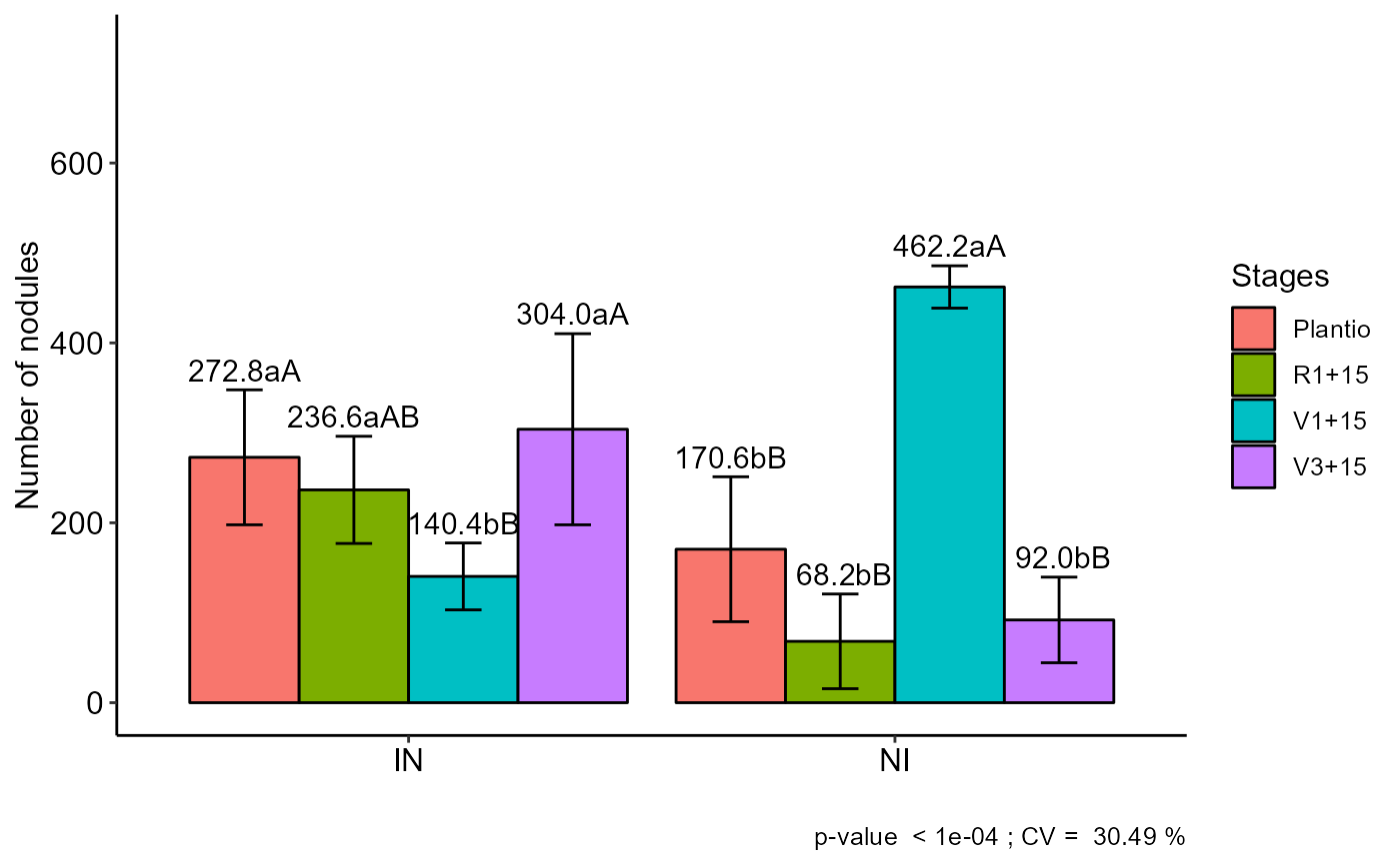
FAT2DBC(f1, f2, bloco, resp, ylab="Number of nodules", legend = "Stages")
#>
#> -----------------------------------------------------------------
#> Normality of errors
#> -----------------------------------------------------------------
#> Method Statistic p.value
#> Shapiro-Wilk normality test(W) 0.9548911 0.1117923
#>
#> As the calculated p-value is greater than the 5% significance level, hypothesis H0 is not rejected. Therefore, errors can be considered normal
#>
#> -----------------------------------------------------------------
#> Homogeneity of Variances
#> -----------------------------------------------------------------
#> Method Statistic p.value
#> Bartlett test(Bartlett's K-squared) 16.11086 0.02412261
#>
#> As the calculated p-value is less than the 5% significance level, H0 is rejected. Therefore, the variances are not homogeneous
#>
#> -----------------------------------------------------------------
#> Independence from errors
#> -----------------------------------------------------------------
#> Method Statistic p.value
#> Durbin-Watson test(DW) 2.050729 0.179264
#>
#> As the calculated p-value is greater than the 5% significance level, hypothesis H0 is not rejected. Therefore, errors can be considered independent
#>
#> -----------------------------------------------------------------
#> Additional Information
#> -----------------------------------------------------------------
#>
#> CV (%) = 30.49
#> Mean = 218.35
#> Median = 185
#> Possible outliers = No discrepant point
#>
#> -----------------------------------------------------------------
#> Analysis of Variance
#> -----------------------------------------------------------------
#> Df Sum Sq Mean.Sq F value Pr(F)
#> Fator1 1 16160.4 16160.400 3.6462291 6.649143e-02
#> Fator2 3 116554.5 38851.500 8.7659631 2.933552e-04
#> bloco 4 11613.6 2903.400 0.6550866 6.282168e-01
#> Fator1:Fator2 3 452096.2 150698.733 34.0017642 1.790168e-09
#> Residuals 28 124098.4 4432.086
#>
#>
#> Your analysis is not valid, suggests using a non-parametric test and try to transform the data
#> -----------------------------------------------------------------
#>
#> Significant interaction: analyzing the interaction
#>
#> -----------------------------------------------------------------
#>
#> -----------------------------------------------------------------
#> Analyzing F1 inside of each level of F2
#> -----------------------------------------------------------------
#> Df Sum Sq Mean Sq F value Pr(>F)
#> bloco 4 11614 2903 0.6551 0.6282168
#> Fator2 3 116554 38851 8.7660 0.0002934 ***
#> Fator2:Fator1 4 468257 117064 26.4129 3.786e-09 ***
#> Fator2:Fator1: Plantio 1 26112 26112 5.8916 0.0218981 *
#> Fator2:Fator1: R1+15 1 70896 70896 15.9962 0.0004207 ***
#> Fator2:Fator1: V1+15 1 258888 258888 58.4123 2.518e-08 ***
#> Fator2:Fator1: V3+15 1 112360 112360 25.3515 2.520e-05 ***
#> Residuals 28 124098 4432
#> ---
#> Signif. codes: 0 '***' 0.001 '**' 0.01 '*' 0.05 '.' 0.1 ' ' 1
#>
#> -----------------------------------------------------------------
#> Analyzing F2 inside of the level of F1
#> -----------------------------------------------------------------
#>
#> Df Sum Sq Mean Sq F value Pr(>F)
#> bloco 4 11614 2903 0.6551 0.628217
#> Fator1 1 16160 16160 3.6462 0.066491 .
#> Fator1:Fator2 6 568651 94775 21.3839 2.917e-09 ***
#> Fator1:Fator2: IN 3 75470 25157 5.6760 0.003625 **
#> Fator1:Fator2: NI 3 493181 164394 37.0917 6.882e-10 ***
#> Residuals 28 124098 4432
#> ---
#> Signif. codes: 0 '***' 0.001 '**' 0.01 '*' 0.05 '.' 0.1 ' ' 1
#>
#> -----------------------------------------------------------------
#> Final table
#> -----------------------------------------------------------------
#> Plantio R1+15 V1+15 V3+15
#> IN 272.8 aA 236.6 aAB 140.4 bB 304.0 aA
#> NI 170.6 bB 68.2 bB 462.2 aA 92.0 bB
#>
#>
#> Averages followed by the same lowercase letter in the column
#> and uppercase in the row do not differ by the tukey (p< 0.05 )
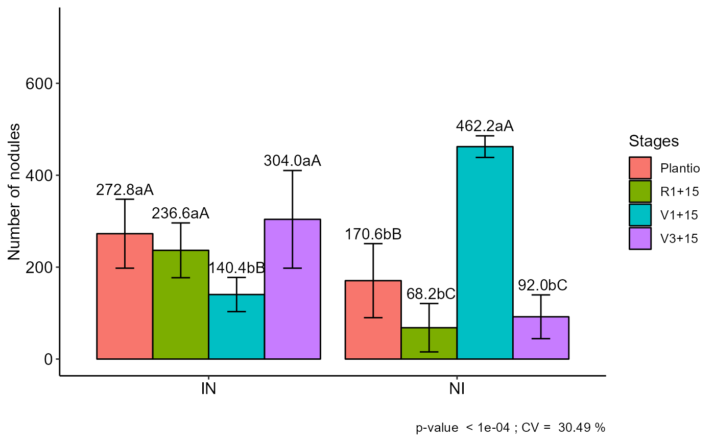
 FAT2DBC(f1, f2, bloco, resp, mcomp="sk", ylab="Number of nodules", legend = "Stages")
#>
#> -----------------------------------------------------------------
#> Normality of errors
#> -----------------------------------------------------------------
#> Method Statistic p.value
#> Shapiro-Wilk normality test(W) 0.9548911 0.1117923
#>
#> As the calculated p-value is greater than the 5% significance level, hypothesis H0 is not rejected. Therefore, errors can be considered normal
#>
#> -----------------------------------------------------------------
#> Homogeneity of Variances
#> -----------------------------------------------------------------
#> Method Statistic p.value
#> Bartlett test(Bartlett's K-squared) 16.11086 0.02412261
#>
#> As the calculated p-value is less than the 5% significance level, H0 is rejected. Therefore, the variances are not homogeneous
#>
#> -----------------------------------------------------------------
#> Independence from errors
#> -----------------------------------------------------------------
#> Method Statistic p.value
#> Durbin-Watson test(DW) 2.050729 0.179264
#>
#> As the calculated p-value is greater than the 5% significance level, hypothesis H0 is not rejected. Therefore, errors can be considered independent
#>
#> -----------------------------------------------------------------
#> Additional Information
#> -----------------------------------------------------------------
#>
#> CV (%) = 30.49
#> Mean = 218.35
#> Median = 185
#> Possible outliers = No discrepant point
#>
#> -----------------------------------------------------------------
#> Analysis of Variance
#> -----------------------------------------------------------------
#> Df Sum Sq Mean.Sq F value Pr(F)
#> Fator1 1 16160.4 16160.400 3.6462291 6.649143e-02
#> Fator2 3 116554.5 38851.500 8.7659631 2.933552e-04
#> bloco 4 11613.6 2903.400 0.6550866 6.282168e-01
#> Fator1:Fator2 3 452096.2 150698.733 34.0017642 1.790168e-09
#> Residuals 28 124098.4 4432.086
#>
#>
#> Your analysis is not valid, suggests using a non-parametric test and try to transform the data
#> -----------------------------------------------------------------
#>
#> Significant interaction: analyzing the interaction
#>
#> -----------------------------------------------------------------
#>
#> -----------------------------------------------------------------
#> Analyzing F1 inside of each level of F2
#> -----------------------------------------------------------------
#> Df Sum Sq Mean Sq F value Pr(>F)
#> bloco 4 11614 2903 0.6551 0.6282168
#> Fator2 3 116554 38851 8.7660 0.0002934 ***
#> Fator2:Fator1 4 468257 117064 26.4129 3.786e-09 ***
#> Fator2:Fator1: Plantio 1 26112 26112 5.8916 0.0218981 *
#> Fator2:Fator1: R1+15 1 70896 70896 15.9962 0.0004207 ***
#> Fator2:Fator1: V1+15 1 258888 258888 58.4123 2.518e-08 ***
#> Fator2:Fator1: V3+15 1 112360 112360 25.3515 2.520e-05 ***
#> Residuals 28 124098 4432
#> ---
#> Signif. codes: 0 '***' 0.001 '**' 0.01 '*' 0.05 '.' 0.1 ' ' 1
#>
#> -----------------------------------------------------------------
#> Analyzing F2 inside of the level of F1
#> -----------------------------------------------------------------
#>
#> Df Sum Sq Mean Sq F value Pr(>F)
#> bloco 4 11614 2903 0.6551 0.628217
#> Fator1 1 16160 16160 3.6462 0.066491 .
#> Fator1:Fator2 6 568651 94775 21.3839 2.917e-09 ***
#> Fator1:Fator2: IN 3 75470 25157 5.6760 0.003625 **
#> Fator1:Fator2: NI 3 493181 164394 37.0917 6.882e-10 ***
#> Residuals 28 124098 4432
#> ---
#> Signif. codes: 0 '***' 0.001 '**' 0.01 '*' 0.05 '.' 0.1 ' ' 1
#>
#> -----------------------------------------------------------------
#> Final table
#> -----------------------------------------------------------------
#> Plantio R1+15 V1+15 V3+15
#> IN 272.8 aA 236.6 aA 140.4 bB 304.0 aA
#> NI 170.6 bB 68.2 bC 462.2 aA 92.0 bC
#>
#>
#> Averages followed by the same lowercase letter in the column
#> and uppercase in the row do not differ by the sk (p< 0.05 )
FAT2DBC(f1, f2, bloco, resp, mcomp="sk", ylab="Number of nodules", legend = "Stages")
#>
#> -----------------------------------------------------------------
#> Normality of errors
#> -----------------------------------------------------------------
#> Method Statistic p.value
#> Shapiro-Wilk normality test(W) 0.9548911 0.1117923
#>
#> As the calculated p-value is greater than the 5% significance level, hypothesis H0 is not rejected. Therefore, errors can be considered normal
#>
#> -----------------------------------------------------------------
#> Homogeneity of Variances
#> -----------------------------------------------------------------
#> Method Statistic p.value
#> Bartlett test(Bartlett's K-squared) 16.11086 0.02412261
#>
#> As the calculated p-value is less than the 5% significance level, H0 is rejected. Therefore, the variances are not homogeneous
#>
#> -----------------------------------------------------------------
#> Independence from errors
#> -----------------------------------------------------------------
#> Method Statistic p.value
#> Durbin-Watson test(DW) 2.050729 0.179264
#>
#> As the calculated p-value is greater than the 5% significance level, hypothesis H0 is not rejected. Therefore, errors can be considered independent
#>
#> -----------------------------------------------------------------
#> Additional Information
#> -----------------------------------------------------------------
#>
#> CV (%) = 30.49
#> Mean = 218.35
#> Median = 185
#> Possible outliers = No discrepant point
#>
#> -----------------------------------------------------------------
#> Analysis of Variance
#> -----------------------------------------------------------------
#> Df Sum Sq Mean.Sq F value Pr(F)
#> Fator1 1 16160.4 16160.400 3.6462291 6.649143e-02
#> Fator2 3 116554.5 38851.500 8.7659631 2.933552e-04
#> bloco 4 11613.6 2903.400 0.6550866 6.282168e-01
#> Fator1:Fator2 3 452096.2 150698.733 34.0017642 1.790168e-09
#> Residuals 28 124098.4 4432.086
#>
#>
#> Your analysis is not valid, suggests using a non-parametric test and try to transform the data
#> -----------------------------------------------------------------
#>
#> Significant interaction: analyzing the interaction
#>
#> -----------------------------------------------------------------
#>
#> -----------------------------------------------------------------
#> Analyzing F1 inside of each level of F2
#> -----------------------------------------------------------------
#> Df Sum Sq Mean Sq F value Pr(>F)
#> bloco 4 11614 2903 0.6551 0.6282168
#> Fator2 3 116554 38851 8.7660 0.0002934 ***
#> Fator2:Fator1 4 468257 117064 26.4129 3.786e-09 ***
#> Fator2:Fator1: Plantio 1 26112 26112 5.8916 0.0218981 *
#> Fator2:Fator1: R1+15 1 70896 70896 15.9962 0.0004207 ***
#> Fator2:Fator1: V1+15 1 258888 258888 58.4123 2.518e-08 ***
#> Fator2:Fator1: V3+15 1 112360 112360 25.3515 2.520e-05 ***
#> Residuals 28 124098 4432
#> ---
#> Signif. codes: 0 '***' 0.001 '**' 0.01 '*' 0.05 '.' 0.1 ' ' 1
#>
#> -----------------------------------------------------------------
#> Analyzing F2 inside of the level of F1
#> -----------------------------------------------------------------
#>
#> Df Sum Sq Mean Sq F value Pr(>F)
#> bloco 4 11614 2903 0.6551 0.628217
#> Fator1 1 16160 16160 3.6462 0.066491 .
#> Fator1:Fator2 6 568651 94775 21.3839 2.917e-09 ***
#> Fator1:Fator2: IN 3 75470 25157 5.6760 0.003625 **
#> Fator1:Fator2: NI 3 493181 164394 37.0917 6.882e-10 ***
#> Residuals 28 124098 4432
#> ---
#> Signif. codes: 0 '***' 0.001 '**' 0.01 '*' 0.05 '.' 0.1 ' ' 1
#>
#> -----------------------------------------------------------------
#> Final table
#> -----------------------------------------------------------------
#> Plantio R1+15 V1+15 V3+15
#> IN 272.8 aA 236.6 aA 140.4 bB 304.0 aA
#> NI 170.6 bB 68.2 bC 462.2 aA 92.0 bC
#>
#>
#> Averages followed by the same lowercase letter in the column
#> and uppercase in the row do not differ by the sk (p< 0.05 )
 #================================================
# Example covercrops
#================================================
library(AgroR)
data(covercrops)
attach(covercrops)
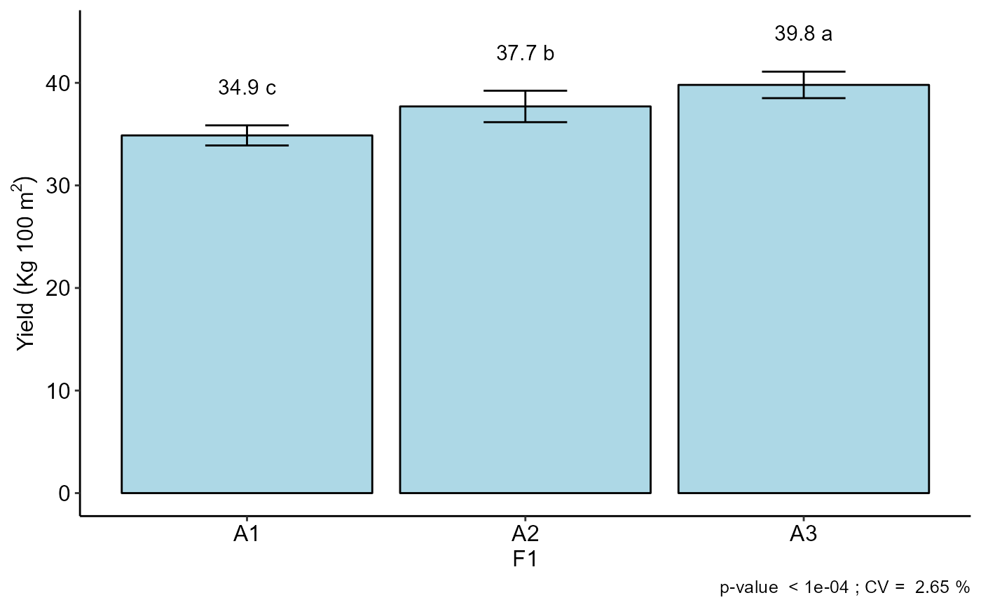
FAT2DBC(A, B, Bloco, Resp, ylab=expression("Yield"~(Kg~"100 m"^2)),
legend = "Cover crops")
#>
#> -----------------------------------------------------------------
#> Normality of errors
#> -----------------------------------------------------------------
#> Method Statistic p.value
#> Shapiro-Wilk normality test(W) 0.9758908 0.6061712
#>
#> As the calculated p-value is greater than the 5% significance level, hypothesis H0 is not rejected. Therefore, errors can be considered normal
#>
#> -----------------------------------------------------------------
#> Homogeneity of Variances
#> -----------------------------------------------------------------
#> Method Statistic p.value
#> Bartlett test(Bartlett's K-squared) 10.19232 0.2517862
#>
#> As the calculated p-value is greater than the 5% significance level, hypothesis H0 is not rejected. Therefore, the variances can be considered homogeneous
#>
#> -----------------------------------------------------------------
#> Independence from errors
#> -----------------------------------------------------------------
#> Method Statistic p.value
#> Durbin-Watson test(DW) 2.335214 0.3781148
#>
#> As the calculated p-value is greater than the 5% significance level, hypothesis H0 is not rejected. Therefore, errors can be considered independent
#>
#> -----------------------------------------------------------------
#> Additional Information
#> -----------------------------------------------------------------
#>
#> CV (%) = 2.65
#> Mean = 37.4583
#> Median = 37.45
#> Possible outliers = No discrepant point
#>
#> -----------------------------------------------------------------
#> Analysis of Variance
#> -----------------------------------------------------------------
#> Df Sum Sq Mean.Sq F value Pr(F)
#> Fator1 2 146.585000 73.292500 74.645449 4.979960e-11
#> Fator2 2 23.021667 11.510833 11.723318 2.805884e-04
#> bloco 3 2.167500 0.722500 0.735837 5.409183e-01
#> Fator1:Fator2 4 6.008333 1.502083 1.529811 2.252749e-01
#> Residuals 24 23.565000 0.981875
#>
#> -----------------------------------------------------------------
#> No significant interaction
#> -----------------------------------------------------------------
#>
#> -----------------------------------------------------------------
#> F1
#> -----------------------------------------------------------------
#> Multiple Comparison Test: Tukey HSD
#> resp groups
#> A3 39.800 a
#> A2 37.700 b
#> A1 34.875 c
#>
#>
#>
#> -----------------------------------------------------------------
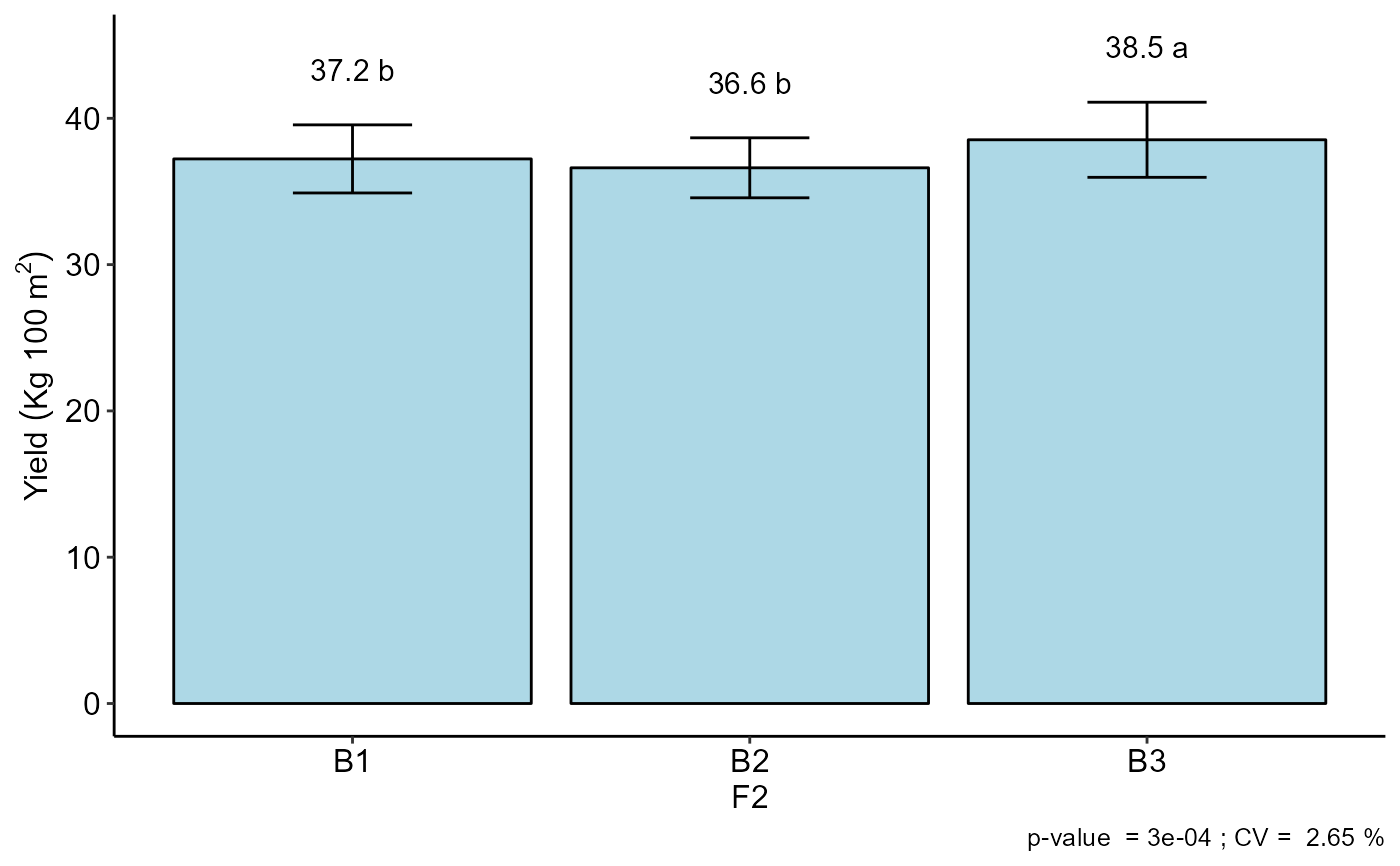
#> F2
#> -----------------------------------------------------------------
#> Multiple Comparison Test: Tukey HSD
#> resp groups
#> B3 38.53333 a
#> B1 37.22500 b
#> B2 36.61667 b
#>
#>
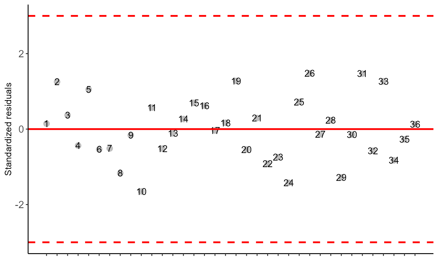
#> $residplot
#================================================
# Example covercrops
#================================================
library(AgroR)
data(covercrops)
attach(covercrops)
FAT2DBC(A, B, Bloco, Resp, ylab=expression("Yield"~(Kg~"100 m"^2)),
legend = "Cover crops")
#>
#> -----------------------------------------------------------------
#> Normality of errors
#> -----------------------------------------------------------------
#> Method Statistic p.value
#> Shapiro-Wilk normality test(W) 0.9758908 0.6061712
#>
#> As the calculated p-value is greater than the 5% significance level, hypothesis H0 is not rejected. Therefore, errors can be considered normal
#>
#> -----------------------------------------------------------------
#> Homogeneity of Variances
#> -----------------------------------------------------------------
#> Method Statistic p.value
#> Bartlett test(Bartlett's K-squared) 10.19232 0.2517862
#>
#> As the calculated p-value is greater than the 5% significance level, hypothesis H0 is not rejected. Therefore, the variances can be considered homogeneous
#>
#> -----------------------------------------------------------------
#> Independence from errors
#> -----------------------------------------------------------------
#> Method Statistic p.value
#> Durbin-Watson test(DW) 2.335214 0.3781148
#>
#> As the calculated p-value is greater than the 5% significance level, hypothesis H0 is not rejected. Therefore, errors can be considered independent
#>
#> -----------------------------------------------------------------
#> Additional Information
#> -----------------------------------------------------------------
#>
#> CV (%) = 2.65
#> Mean = 37.4583
#> Median = 37.45
#> Possible outliers = No discrepant point
#>
#> -----------------------------------------------------------------
#> Analysis of Variance
#> -----------------------------------------------------------------
#> Df Sum Sq Mean.Sq F value Pr(F)
#> Fator1 2 146.585000 73.292500 74.645449 4.979960e-11
#> Fator2 2 23.021667 11.510833 11.723318 2.805884e-04
#> bloco 3 2.167500 0.722500 0.735837 5.409183e-01
#> Fator1:Fator2 4 6.008333 1.502083 1.529811 2.252749e-01
#> Residuals 24 23.565000 0.981875
#>
#> -----------------------------------------------------------------
#> No significant interaction
#> -----------------------------------------------------------------
#>
#> -----------------------------------------------------------------
#> F1
#> -----------------------------------------------------------------
#> Multiple Comparison Test: Tukey HSD
#> resp groups
#> A3 39.800 a
#> A2 37.700 b
#> A1 34.875 c
#>
#>
#>
#> -----------------------------------------------------------------
#> F2
#> -----------------------------------------------------------------
#> Multiple Comparison Test: Tukey HSD
#> resp groups
#> B3 38.53333 a
#> B1 37.22500 b
#> B2 36.61667 b
#>
#>
#> $residplot
 #>
#> $graph1
#>
#> $graph1
 #>
#> $graph2
#>
#> $graph2
 #>
FAT2DBC(A, B, Bloco, Resp, mcomp="sk", ylab=expression("Yield"~(Kg~"100 m"^2)),
legend = "Cover crops")
#>
#> -----------------------------------------------------------------
#> Normality of errors
#> -----------------------------------------------------------------
#> Method Statistic p.value
#> Shapiro-Wilk normality test(W) 0.9758908 0.6061712
#>
#> As the calculated p-value is greater than the 5% significance level, hypothesis H0 is not rejected. Therefore, errors can be considered normal
#>
#> -----------------------------------------------------------------
#> Homogeneity of Variances
#> -----------------------------------------------------------------
#> Method Statistic p.value
#> Bartlett test(Bartlett's K-squared) 10.19232 0.2517862
#>
#> As the calculated p-value is greater than the 5% significance level, hypothesis H0 is not rejected. Therefore, the variances can be considered homogeneous
#>
#> -----------------------------------------------------------------
#> Independence from errors
#> -----------------------------------------------------------------
#> Method Statistic p.value
#> Durbin-Watson test(DW) 2.335214 0.3781148
#>
#> As the calculated p-value is greater than the 5% significance level, hypothesis H0 is not rejected. Therefore, errors can be considered independent
#>
#> -----------------------------------------------------------------
#> Additional Information
#> -----------------------------------------------------------------
#>
#> CV (%) = 2.65
#> Mean = 37.4583
#> Median = 37.45
#> Possible outliers = No discrepant point
#>
#> -----------------------------------------------------------------
#> Analysis of Variance
#> -----------------------------------------------------------------
#> Df Sum Sq Mean.Sq F value Pr(F)
#> Fator1 2 146.585000 73.292500 74.645449 4.979960e-11
#> Fator2 2 23.021667 11.510833 11.723318 2.805884e-04
#> bloco 3 2.167500 0.722500 0.735837 5.409183e-01
#> Fator1:Fator2 4 6.008333 1.502083 1.529811 2.252749e-01
#> Residuals 24 23.565000 0.981875
#>
#> -----------------------------------------------------------------
#> No significant interaction
#> -----------------------------------------------------------------
#>
#> -----------------------------------------------------------------
#> F1
#> -----------------------------------------------------------------
#> Multiple Comparison Test: Scott-Knott
#> resp groups
#> A3 39.800 a
#> A2 37.700 b
#> A1 34.875 c
#>
#>
#>
#> -----------------------------------------------------------------
#> F2
#> -----------------------------------------------------------------
#> Multiple Comparison Test: Scott-Knott
#> resp groups
#> B3 38.53333 a
#> B1 37.22500 b
#> B2 36.61667 b
#>
#>
#> $residplot
#>
FAT2DBC(A, B, Bloco, Resp, mcomp="sk", ylab=expression("Yield"~(Kg~"100 m"^2)),
legend = "Cover crops")
#>
#> -----------------------------------------------------------------
#> Normality of errors
#> -----------------------------------------------------------------
#> Method Statistic p.value
#> Shapiro-Wilk normality test(W) 0.9758908 0.6061712
#>
#> As the calculated p-value is greater than the 5% significance level, hypothesis H0 is not rejected. Therefore, errors can be considered normal
#>
#> -----------------------------------------------------------------
#> Homogeneity of Variances
#> -----------------------------------------------------------------
#> Method Statistic p.value
#> Bartlett test(Bartlett's K-squared) 10.19232 0.2517862
#>
#> As the calculated p-value is greater than the 5% significance level, hypothesis H0 is not rejected. Therefore, the variances can be considered homogeneous
#>
#> -----------------------------------------------------------------
#> Independence from errors
#> -----------------------------------------------------------------
#> Method Statistic p.value
#> Durbin-Watson test(DW) 2.335214 0.3781148
#>
#> As the calculated p-value is greater than the 5% significance level, hypothesis H0 is not rejected. Therefore, errors can be considered independent
#>
#> -----------------------------------------------------------------
#> Additional Information
#> -----------------------------------------------------------------
#>
#> CV (%) = 2.65
#> Mean = 37.4583
#> Median = 37.45
#> Possible outliers = No discrepant point
#>
#> -----------------------------------------------------------------
#> Analysis of Variance
#> -----------------------------------------------------------------
#> Df Sum Sq Mean.Sq F value Pr(F)
#> Fator1 2 146.585000 73.292500 74.645449 4.979960e-11
#> Fator2 2 23.021667 11.510833 11.723318 2.805884e-04
#> bloco 3 2.167500 0.722500 0.735837 5.409183e-01
#> Fator1:Fator2 4 6.008333 1.502083 1.529811 2.252749e-01
#> Residuals 24 23.565000 0.981875
#>
#> -----------------------------------------------------------------
#> No significant interaction
#> -----------------------------------------------------------------
#>
#> -----------------------------------------------------------------
#> F1
#> -----------------------------------------------------------------
#> Multiple Comparison Test: Scott-Knott
#> resp groups
#> A3 39.800 a
#> A2 37.700 b
#> A1 34.875 c
#>
#>
#>
#> -----------------------------------------------------------------
#> F2
#> -----------------------------------------------------------------
#> Multiple Comparison Test: Scott-Knott
#> resp groups
#> B3 38.53333 a
#> B1 37.22500 b
#> B2 36.61667 b
#>
#>
#> $residplot
 #>
#> $graph1
#>
#> $graph1
 #>
#> $graph2
#>
#> $graph2
 #>
#>