Analysis: Completely randomized design evaluated over time
DICT.RdFunction of the AgroR package for the analysis of experiments conducted in a completely randomized, qualitative, uniform qualitative design with multiple assessments over time, however without considering time as a factor.
DICT(
  trat,
  time,
  response,
  alpha.f = 0.05,
  alpha.t = 0.05,
  mcomp = "tukey",
  theme = theme_classic(),
  geom = "bar",
  xlab = "Independent",
  ylab = "Response",
  p.adj = "holm",
  dec = 3,
  fill = "gray",
  error = TRUE,
  textsize = 12,
  labelsize = 5,
  pointsize = 4.5,
  family = "sans",
  sup = 0,
  addmean = FALSE,
  legend = "Legend",
  ylim = NA,
  width.bar = 0.2,
  size.bar = 0.8,
  posi = c(0.1, 0.8),
  xnumeric = FALSE,
  all.letters = FALSE
)
Arguments
- trat
Numerical or complex vector with treatments
- time
Numerical or complex vector with times
- response
Numerical vector containing the response of the experiment.
- alpha.f
Level of significance of the F test (default is 0.05)
- alpha.t
Significance level of the multiple comparison test (default is 0.05)
- mcomp
Multiple comparison test (Tukey (default), LSD ("lsd"), Scott-Knott ("sk"), Duncan ("duncan") and Kruskal-Wallis ("kw"))
- theme
ggplot2 theme (default is theme_classic())
- geom
Graph type (columns - "bar" or segments "point")
- xlab
treatments name (Accepts the expression() function)
- ylab
Variable response name (Accepts the expression() function)
- p.adj
Method for adjusting p values for Kruskal-Wallis ("none","holm","hommel", "hochberg", "bonferroni", "BH", "BY", "fdr")
- dec
Number of cells
- fill
Defines chart color (to generate different colors for different treatments, define fill = "trat")
- error
Add error bar
- textsize
Font size of the texts and titles of the axes
- labelsize
Font size of the labels
- pointsize
Point size
- family
Font family
- sup
Number of units above the standard deviation or average bar on the graph
- addmean
Plot the average value on the graph (default is TRUE)
- legend
Legend title
- ylim
Define a numerical sequence referring to the y scale. You can use a vector or the `seq` command.
- width.bar
width error bar
- size.bar
size error bar
- posi
Legend position
- xnumeric
Declare x as numeric (default is FALSE)
- all.letters
Adds all label letters regardless of whether it is significant or not.
Value
The function returns the p-value of Anova, the assumptions of normality of errors, homogeneity of variances and independence of errors, multiple comparison test, as well as a line graph
Note
The ordering of the graph is according to the sequence in which the factor levels are arranged in the data sheet. The bars of the column and segment graphs are standard deviation.
References
Principles and procedures of statistics a biometrical approach Steel, Torry and Dickey. Third Edition 1997
Multiple comparisons theory and methods. Departament of statistics the Ohio State University. USA, 1996. Jason C. Hsu. Chapman Hall/CRC.
Practical Nonparametrics Statistics. W.J. Conover, 1999
Ramalho M.A.P., Ferreira D.F., Oliveira A.C. 2000. Experimentacao em Genetica e Melhoramento de Plantas. Editora UFLA.
Scott R.J., Knott M. 1974. A cluster analysis method for grouping mans in the analysis of variance. Biometrics, 30, 507-512.
Examples
rm(list=ls())
data(simulate1)
attach(simulate1)
#> The following objects are masked from aristolochia (pos = 3):
#>
#> resp, trat
#> The following objects are masked from simulate2:
#>
#> resp, tempo, trat
#> The following objects are masked from laranja:
#>
#> resp, trat
#> The following objects are masked from aristolochia (pos = 6):
#>
#> resp, trat
#> The following object is masked from cloro:
#>
#> resp
#> The following object is masked from passiflora:
#>
#> trat
with(simulate1, DICT(trat, tempo, resp))
#>
#> -----------------------------------------------------------------
#> ANOVA and assumptions
#> -----------------------------------------------------------------
#> p-value ANOVA Shapiro-Wilk Bartlett Durbin-Watson CV (%)
#> 1 9.143052e-05 0.44610417 0.23369500 0.2379509 11.625285
#> 2 3.821815e-07 0.93845028 0.30786895 0.6600467 4.163316
#> 3 7.822709e-05 0.59104221 0.46541352 0.3244232 4.189412
#> 4 1.496061e-02 0.09984009 0.09849058 0.1332682 6.462590
#> 5 1.757687e-04 0.67552390 0.42726077 0.3008609 2.566743
#> 6 1.138255e-04 0.70461554 0.37578092 0.6357482 2.093636
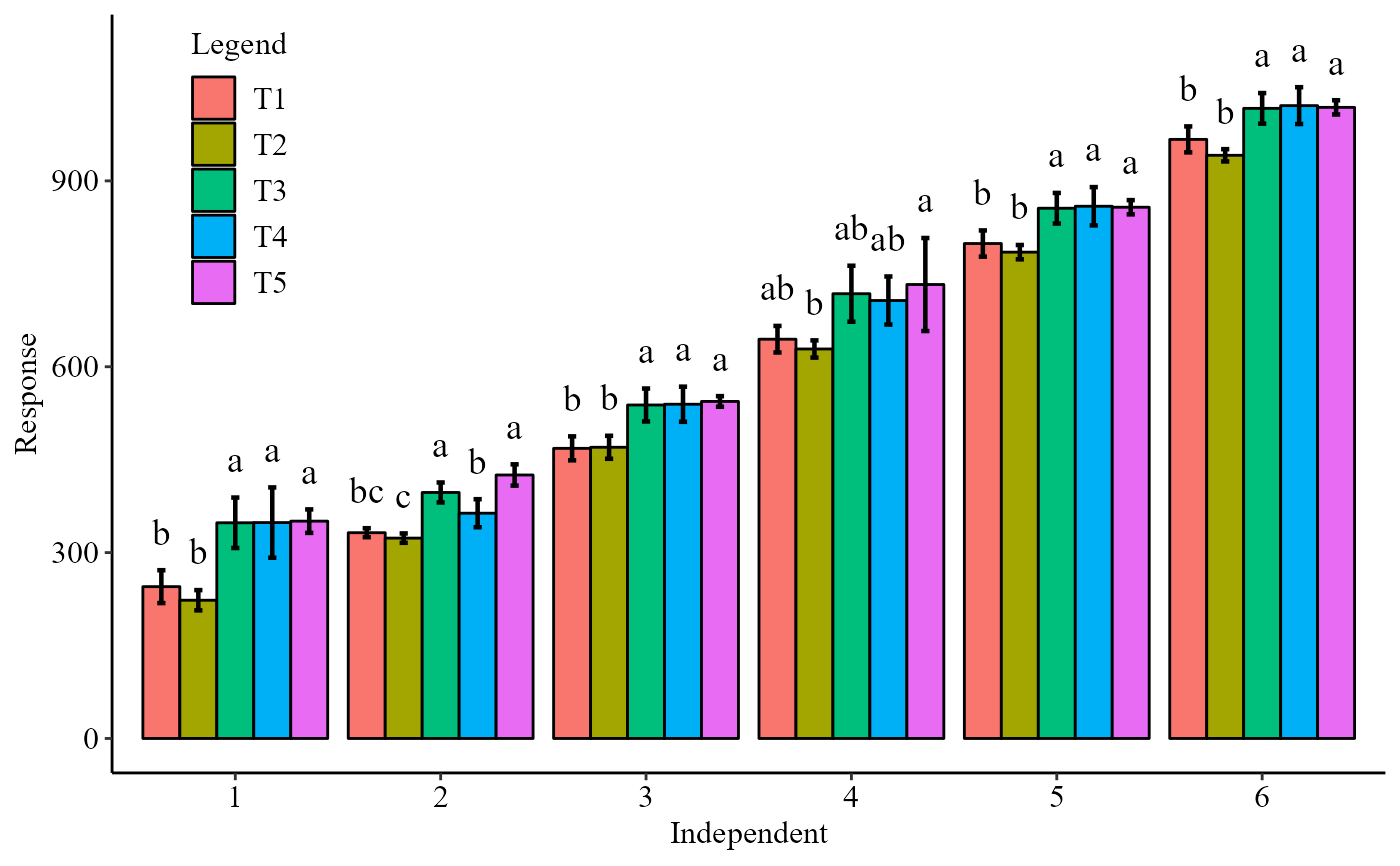
 with(simulate1, DICT(trat, tempo, resp, fill="rainbow",family="serif"))
#>
#> -----------------------------------------------------------------
#> ANOVA and assumptions
#> -----------------------------------------------------------------
#> p-value ANOVA Shapiro-Wilk Bartlett Durbin-Watson CV (%)
#> 1 9.143052e-05 0.44610417 0.23369500 0.2379509 11.625285
#> 2 3.821815e-07 0.93845028 0.30786895 0.6600467 4.163316
#> 3 7.822709e-05 0.59104221 0.46541352 0.3244232 4.189412
#> 4 1.496061e-02 0.09984009 0.09849058 0.1332682 6.462590
#> 5 1.757687e-04 0.67552390 0.42726077 0.3008609 2.566743
#> 6 1.138255e-04 0.70461554 0.37578092 0.6357482 2.093636
with(simulate1, DICT(trat, tempo, resp, fill="rainbow",family="serif"))
#>
#> -----------------------------------------------------------------
#> ANOVA and assumptions
#> -----------------------------------------------------------------
#> p-value ANOVA Shapiro-Wilk Bartlett Durbin-Watson CV (%)
#> 1 9.143052e-05 0.44610417 0.23369500 0.2379509 11.625285
#> 2 3.821815e-07 0.93845028 0.30786895 0.6600467 4.163316
#> 3 7.822709e-05 0.59104221 0.46541352 0.3244232 4.189412
#> 4 1.496061e-02 0.09984009 0.09849058 0.1332682 6.462590
#> 5 1.757687e-04 0.67552390 0.42726077 0.3008609 2.566743
#> 6 1.138255e-04 0.70461554 0.37578092 0.6357482 2.093636
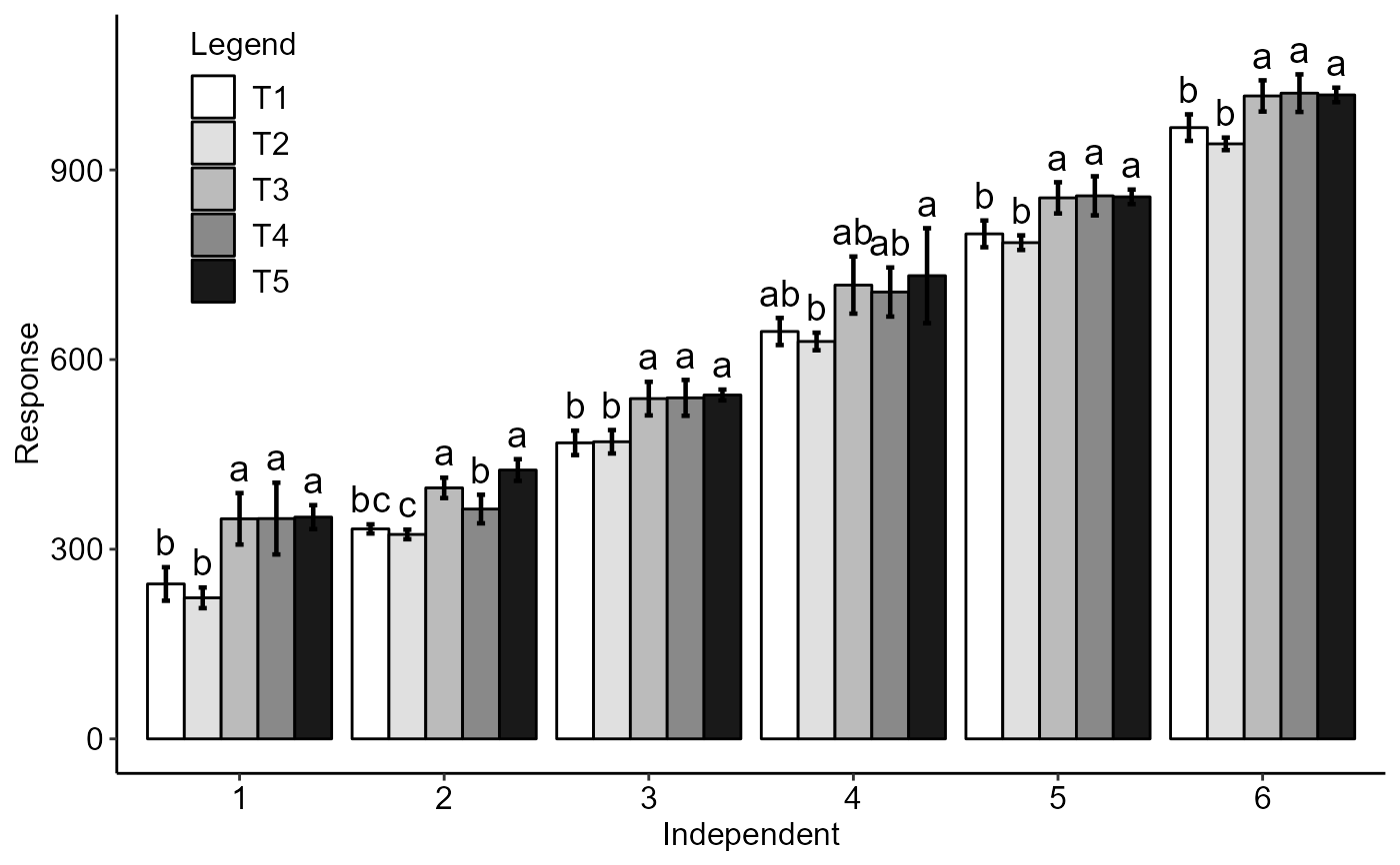
 with(simulate1, DICT(trat, tempo, resp,geom="bar",sup=40))
#>
#> -----------------------------------------------------------------
#> ANOVA and assumptions
#> -----------------------------------------------------------------
#> p-value ANOVA Shapiro-Wilk Bartlett Durbin-Watson CV (%)
#> 1 9.143052e-05 0.44610417 0.23369500 0.2379509 11.625285
#> 2 3.821815e-07 0.93845028 0.30786895 0.6600467 4.163316
#> 3 7.822709e-05 0.59104221 0.46541352 0.3244232 4.189412
#> 4 1.496061e-02 0.09984009 0.09849058 0.1332682 6.462590
#> 5 1.757687e-04 0.67552390 0.42726077 0.3008609 2.566743
#> 6 1.138255e-04 0.70461554 0.37578092 0.6357482 2.093636
with(simulate1, DICT(trat, tempo, resp,geom="bar",sup=40))
#>
#> -----------------------------------------------------------------
#> ANOVA and assumptions
#> -----------------------------------------------------------------
#> p-value ANOVA Shapiro-Wilk Bartlett Durbin-Watson CV (%)
#> 1 9.143052e-05 0.44610417 0.23369500 0.2379509 11.625285
#> 2 3.821815e-07 0.93845028 0.30786895 0.6600467 4.163316
#> 3 7.822709e-05 0.59104221 0.46541352 0.3244232 4.189412
#> 4 1.496061e-02 0.09984009 0.09849058 0.1332682 6.462590
#> 5 1.757687e-04 0.67552390 0.42726077 0.3008609 2.566743
#> 6 1.138255e-04 0.70461554 0.37578092 0.6357482 2.093636
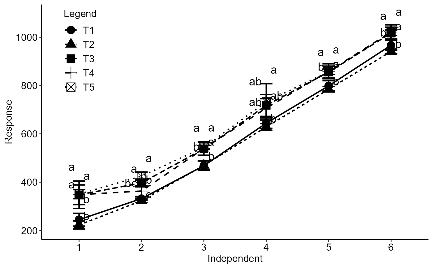
 with(simulate1, DICT(trat, tempo, resp,geom="point",sup=40))
#>
#> -----------------------------------------------------------------
#> ANOVA and assumptions
#> -----------------------------------------------------------------
#> p-value ANOVA Shapiro-Wilk Bartlett Durbin-Watson CV (%)
#> 1 9.143052e-05 0.44610417 0.23369500 0.2379509 11.625285
#> 2 3.821815e-07 0.93845028 0.30786895 0.6600467 4.163316
#> 3 7.822709e-05 0.59104221 0.46541352 0.3244232 4.189412
#> 4 1.496061e-02 0.09984009 0.09849058 0.1332682 6.462590
#> 5 1.757687e-04 0.67552390 0.42726077 0.3008609 2.566743
#> 6 1.138255e-04 0.70461554 0.37578092 0.6357482 2.093636
with(simulate1, DICT(trat, tempo, resp,geom="point",sup=40))
#>
#> -----------------------------------------------------------------
#> ANOVA and assumptions
#> -----------------------------------------------------------------
#> p-value ANOVA Shapiro-Wilk Bartlett Durbin-Watson CV (%)
#> 1 9.143052e-05 0.44610417 0.23369500 0.2379509 11.625285
#> 2 3.821815e-07 0.93845028 0.30786895 0.6600467 4.163316
#> 3 7.822709e-05 0.59104221 0.46541352 0.3244232 4.189412
#> 4 1.496061e-02 0.09984009 0.09849058 0.1332682 6.462590
#> 5 1.757687e-04 0.67552390 0.42726077 0.3008609 2.566743
#> 6 1.138255e-04 0.70461554 0.37578092 0.6357482 2.093636